
Bayesian Inference and the Role of Bayes’ Theorem
Statistical inference is the problem of learning about unknown parameters $\theta$ from observed data $X$. In the frequentist approach, $\theta$ is treated as a fixed but unknown constant, and inference is built around the likelihood $P(X \mid \theta)$ alone.
In the Bayesian approach, $\theta$ is treated as a random variable with its own distribution, and inference is carried out by updating our prior belief $P(\theta)$ after seeing the data — using Bayes’ Theorem to obtain the posterior $P(\theta \mid X)$. This posterior becomes the complete basis for all inference about $\theta$.
Bayes Theorem
Bayes’ Theorem provides a way to update our belief about a parameter $\theta$ after observing data $X$. The formula takes the same form in both the discrete and continuous cases — the only difference is whether the normalizing constant is a sum or an integral.
$$P(\theta \mid X) = \frac{P(X \mid \theta)\, P(\theta)}{P(X)}$$
Where:
- $P(\theta \mid X)$ is the posterior — updated belief about $\theta$ after seeing the data
- $P(X \mid \theta)$ is the likelihood — probability of the data given $\theta$
- $P(\theta)$ is the prior — belief about $\theta$ before seeing the data
- $P(X)$ is the marginal likelihood — a normalizing constant ensuring the posterior sums or integrates to 1
Proof (from Conditional Probability)
Starting from the definition of conditional probability:
$$P(\theta \mid X) = \frac{P(\theta \cap X)}{P(X)}$$
By the definition of joint probability:
$$P(\theta \cap X) = P(X \mid \theta)\, P(\theta)$$
Substituting:
$$P(\theta \mid X) = \frac{P(X \mid \theta)\, P(\theta)}{P(X)}$$
This proof holds for both the discrete and continuous cases.
The Normalizing Constant $P(X)$
The only difference between the discrete and continuous cases lies in how $P(X)$ is computed.
Discrete case — $\theta$ takes values in ${\theta_1, \theta_2, \ldots, \theta_n}$:
$$P(X) = \sum_{i=1}^{n} P(X \mid \theta_i)\, P(\theta_i)$$
Continuous case — $\theta$ is a continuous random variable:
$$P(X) = \int P(X \mid \theta)\, P(\theta)\, d\theta$$
In both cases, $P(X)$ plays the same role: it ensures the posterior is a valid probability distribution.
Why this Theorem is Central to Statistical Inference
The fundamental problem of statistical inference is this: we observe data $X$, but what we truly want to know is $\theta$ — the unknown parameter governing the process that produced the data.
Bayes’ Theorem is the mathematically principled answer to this problem. It tells us exactly how to turn what we observe (the likelihood of the data under each possible $\theta$, and our prior belief about $\theta$) into a complete probability distribution over $\theta$ given the data.
This posterior distribution $P(\theta \mid X)$ encodes our full updated uncertainty about $\theta$. From it we can extract any summary we need: a single best estimate, a measure of spread, or a probability that $\theta$ lies in any region of interest.
In this sense, Bayes’ Theorem is not merely a formula — it is the backbone of statistical inference
Inference on Parameters from a Bayesian Posterior Distribution
In the Bayesian framework, after combining the likelihood and prior using Bayes’ Theorem, the posterior distribution provides a complete description of our updated beliefs about the parameters of interest, given the observed data.
Estimating parameters from the posterior distribution can be done using different methods, each with its own implications and interpretations. Below, we discuss some of the most commonly used methods for parameter estimation in the Bayesian framework.
Discrete Parameter Case
Here we consider the case where the parameter $\theta$ takes values in a finite discrete set ${\theta_1, \theta_2, \ldots, \theta_n}$.
1. Point Estimates
a. Maximum A Posteriori (MAP)
The MAP estimate is the value of $\theta$ with the highest posterior probability:
$$\hat{\theta}_{\text{MAP}_i} =\text{argmax}_{\theta_i}P[\theta_i \mid X]$$
In the discrete case this is simply a scan over all $\theta_i$ — pick the one with the largest posterior mass.
b. Posterior Mean
$$\hat{\theta}_{\text{Mean}}=E[\theta|X]=\sum_{i=1}^{n} \theta_{i} P[\theta_{i}|X]$$
A weighted average of the $\theta_i$ values, weighted by their posterior probabilities.
c. Posterior Median
Sort $\theta_1 < \theta_2 < \cdots < \theta_n$ and build the cumulative posterior (see Section 2). The median is the first $\theta_k$ for which the cumulative mass reaches $\geq 0.5$. It is more robust than the mean when the posterior is skewed.
d. Posterior Variance
$$\text{Var}(\theta \mid X) = \sum_{i=1}^n (\theta_i – \hat{\theta}_{\text{Mean}})^2\, P(\theta_i \mid X)$$
2. The Cumulative Posterior — The Key Tool for Intervals
Assume $\theta_1 < \theta_2 < \cdots < \theta_n$. Define the cumulative posterior:
$$F(\theta_k) = \sum_{i=1}^{k} P(\theta_i \mid X)$$
This is the discrete analog of the CDF. It is the foundation for credible intervals and tail probability statements.
3. Interval Estimates
For a $(1-\alpha)$ credible interval, cut $\alpha/2$ from each tail using the cumulative posterior:
- Lower bound: smallest $\theta_i$ such that $F(\theta_i) \geq \alpha/2$
- Upper bound: smallest $\theta_k$ such that $F(\theta_k) \geq 1 – \alpha/2$
Because $\theta$ is discrete, the actual achieved coverage will generally be $\geq 1-\alpha$, not exactly equal. Always report the achieved coverage alongside the interval.
4. Posterior Probability Statements
The cumulative posterior directly answers questions of the form $P(\theta < c \mid X)$:
$$P(\theta < c \mid X) = \sum_{\theta_i < c} P(\theta_i \mid X)$$
Similarly, $P(\theta \leq c) = F(\theta_k)$ where $\theta_k$ is the largest $\theta_i \leq c$.
The workflow is: build the cumulative table once, then read off any interval or tail probability needed.
After completing the discrete case, we now turn to the continuous case where $\theta$ takes values over a real interval rather than a finite set. The structure of inference remains identical — only the summations are replaced by integrals.
Continuous Parameter Case
Here we consider the case where the parameter $\theta$ is a continuous random variable taking values in a real interval $(a, b)$.
1. Point Estimates
a. Maximum A Posteriori (MAP)
The MAP estimate is the value of $\theta$ that maximizes the posterior density:
$$\hat{\theta}_{\text{MAP}}=\text{argmax}_{\theta}P[\theta|X]$$
This is typically found by differentiating the posterior (or equivalently the log-posterior) and solving for the stationary point.
b. Posterior Mean
$$\hat{\theta}_{mean} = \int_a^b \theta\, P(\theta \mid X)\, d\theta$$
A weighted average of $\theta$ values over the interval, weighted by the posterior density.
c. Posterior Median
The median is the value $\theta_m$ such that $F(\theta_m) = 0.5$, where $F$ is the cumulative posterior (see Section 2). It is more robust than the mean when the posterior is skewed.
d. Posterior Variance
$$\text{Var}(\theta \mid X) = \int_a^b (\theta – \hat{\theta}_{mean})^2\, P(\theta \mid X)\, d\theta$$
2. The Cumulative Posterior — The Key Tool for Intervals
For $\theta \in (a, b)$, define the cumulative posterior:
$$F(t) = \int_a^t P(\theta \mid X)\, d\theta, \quad t \in (a, b)$$
This is the CDF of the posterior distribution. It is the foundation for credible intervals and tail probability statements.
3. Interval Estimates
For a $(1-\alpha)$ credible interval, cut $\alpha/2$ from each tail using the cumulative posterior:
- Lower bound: value $\theta_L$ such that $F(\theta_L) = \alpha/2$
- Upper bound: value $\theta_U$ such that $F(\theta_U) = 1 – \alpha/2$
These are obtained by inverting the CDF, i.e. $\theta_L = F^{-1}(\alpha/2)$ and $\theta_U = F^{-1}(1-\alpha/2)$.
4. Posterior Probability Statements
The cumulative posterior directly answers questions of the form $P(\theta < c \mid X)$:
$$P(\theta < c \mid X) = \int_a^c P(\theta \mid X)\, d\theta = F(c)$$
Similarly, $P(\theta \leq c) = F(c)$ since $\theta$ is continuous.
The workflow is: obtain the CDF once, then read off any interval or tail probability needed.
Conclusions
- For a discrete parameter, the posterior is a probability mass function over a finite set. Every integral in the standard Bayesian formulas is replaced by a sum.
- For a continuous parameter on $(a,b)$, the posterior is a probability density function over a real interval. Every sum in the discrete Bayesian formulas is replaced by an integral.
- All summaries — MAP, mean, median, variance, credible intervals, and tail probabilities — follow directly from the posterior distribution (mass / density) and its cumulative form.
Bayesian Inference — Discrete Parameter
Introductory Example: Probability of Rainfall on January 15
Problem Description
A city’s meteorological record spanning 150 years shows that rain was recorded on January 15 in exactly 23 of those years. A panel of experts, drawing on historical patterns and domain knowledge, believes the true probability of rainfall on that day could be one of four values: 1%, 5%, 10%, or 20%. They assign prior probabilities to each of these values reflecting their collective belief that rainfall is likely rare.
The question is: after seeing the historical data, what should we now believe about the probability of rainfall on January 15?
Prior
The parameter $\theta$ takes values in ${0.01, 0.05, 0.10, 0.20}$ with prior probabilities:
| $\theta$ | P(theta) |
|---|---|
| 0.01 | 0.70 |
| 0.05 | 0.20 |
| 0.10 | 0.07 |
| 0.20 | 0.03 |
The experts assigned a high prior to $\theta = 0.01$, reflecting a belief that rain on this day is uncommon.
Data and Likelihood
The outcome on each January 15 is binary — it either rains or it does not. Over $n = 150$ years, rain was recorded $x = 23$ times. Since the outcome is binary and the number of trials is fixed, the appropriate likelihood is the Binomial distribution:
$$\mathscr{L}(\theta) = P(X = x \mid \theta) = \binom{n}{x}\, \theta^x\, (1-\theta)^{n-x} \quad \text{with } n = 150,\ x = 23$$
Computing the likelihood for each candidate $\theta$:
| theta | Likelihood |
|---|---|
| 0.01 | 0.0000 |
| 0.05 | 0.0000 |
| 0.10 | 0.01133 |
| 0.20 | 0.03031 |
The likelihood is extremely small for $\theta = 0.01$ — the observed data is almost impossible if the true probability of rain is only 1%.
Algorithm: Computing the Posterior
Step 1: Compute the joint probability $P(X \mid \theta_i) \cdot P(\theta_i)$ for each $\theta_i$.
Step 2: Sum across all values to get the normalising constant:
$$P(X) = \sum_i P(X \mid \theta_i)\, P(\theta_i)$$
$$P(X) = (0.70)(2.047 \times 10^{-20}) + (0.20)(1.30 \times 10^{-6}) + (0.07)(0.01133) + (0.03)(0.03031) = 0.00170266$$
Step 3: Apply Bayes’ Theorem for each $\theta_i$:
$$P(\theta_i \mid X) = \frac{P(X \mid \theta_i)\, P(\theta_i)}{P(X)}$$
Posterior Results
| theta | Prior | Posterior |
|---|---|---|
| 0.01 | 0.70 | 0.000 |
| 0.05 | 0.20 | 0.00015 |
| 0.10 | 0.07 | 0.4658 |
| 0.20 | 0.03 | 0.5340 |
Interpretation
The experts began with a strong prior belief that rainfall on January 15 is rare — assigning 70% probability to $\theta = 0.01$. However, the data tells a different story: 23 rainy days out of 150 years is far more consistent with a 10–20% chance of rain. The posterior completely overturns the prior belief, concentrating mass on $\theta = 0.10$ and $\theta = 0.20$.
This is the Bayesian update in action: data can overturn even strongly held prior beliefs when the evidence is clear enough.
—
Main Case Study: Honda vs Hero Mileage Dispute
Honda questioned Hero’s claim that the Splendor iSmart achieves 102.5 km/litre, calling it misleading. Hero countered that the figure was certified by iCAT (International Centre for Automotive Technology). To investigate analytically, iCAT tests a batch of bikes and records mileage data. Depending on what is measured, three different data types arise — each requiring a different likelihood.
Data Type I — Number of Bikes Passing the Test (Binomial)
Problem Description
iCAT tests a fixed batch of $n = 100$ bikes. Each bike either passes the mileage threshold or it does not — a binary outcome. The observed number of bikes that pass the test is $x = 35$. The goal is to estimate $\theta$, the true proportion of bikes that meet the mileage claim.
Prior
Experts assign prior beliefs over five candidate values of $\theta$:
| theta | Prior |
|---|---|
| 0.10 | 0.01 |
| 0.40 | 0.02 |
| 0.50 | 0.52 |
| 0.75 | 0.20 |
| 0.90 | 0.25 |
The prior strongly favours $\theta = 0.50$ — a belief that roughly half the bikes will pass.
Data and Likelihood
Since each bike independently either passes or fails, and the batch size is fixed at $n = 100$, the appropriate likelihood is the Binomial distribution:
$$P(X = x \mid \theta) = \binom{n}{x}\, \theta^x\, (1-\theta)^{n-x} \quad \text{with } n = 100,\ x = 35$$
Algorithm
Step 1: Evaluate $P(X = 35 \mid \theta_i)$ for each candidate $\theta_i$ using the Binomial PMF.
Step 2: Compute the normalising constant:
$$P(X) = \sum_i P(X \mid \theta_i)\, P(\theta_i)$$
Step 3: Apply Bayes’ Theorem:
$$P(\theta_i \mid X) = \frac{P(X \mid \theta_i)\, P(\theta_i)}{P(X)}$$
Posterior Results and Plot
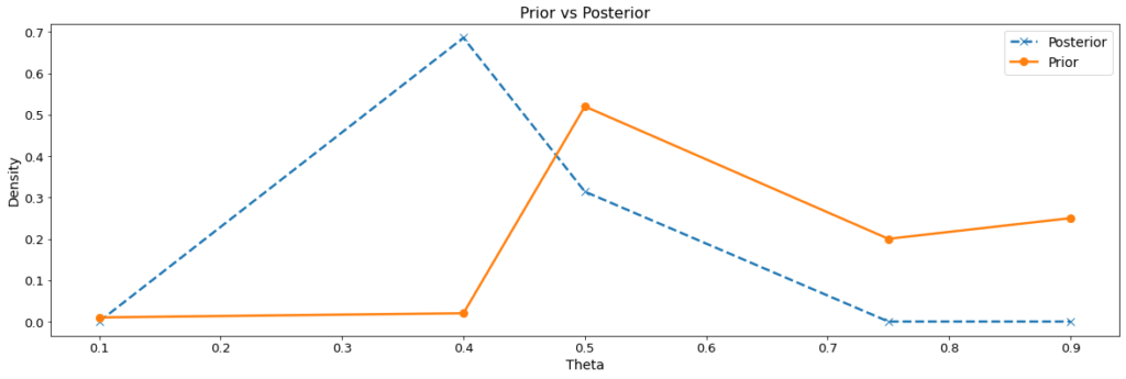
| Parameter $\theta$ | Prior | Posterior |
|---|---|---|
| 0.10 | 0.01 | 0.000 |
| 0.40 | 0.02 | 0.686 |
| 0.50 | 0.52 | 0.314 |
| 0.75 | 0.20 | 0.000 |
| 0.90 | 0.25 | 0.000 |
Interpretation
The prior strongly favoured $\theta = 0.50$ (52% prior probability). But observing only 35 out of 100 bikes passing — a pass rate of 35% — is far more consistent with $\theta = 0.40$. The posterior shifts dramatically: $\theta = 0.40$ receives 68.6% of the posterior mass, while values of 0.75 and 0.90 are essentially ruled out by the data. The data has corrected the prior belief toward a more realistic pass rate.
—
Data Type II — Count of Bikes Passing (Unknown Batch Size, Poisson)
Problem Description
In this scenario, iCAT does not fix the number of bikes to test in advance — testing continues until a natural stopping point. What is recorded is the count of bikes that pass the mileage threshold. Since the batch size is not fixed but the average rate of passing bikes is of interest, the appropriate model is the Poisson distribution, where $\theta$ represents the expected number of bikes passing per batch.
Prior
Experts assign prior beliefs over four candidate values of $\theta$ (expected count):
| theta | Prior |
|---|---|
| 30 | 0.40 |
| 40 | 0.25 |
| 50 | 0.18 |
| 60 | 0.17 |
The prior leans toward $\theta = 30$ — a belief that the expected count of passing bikes is relatively low.
Data and Likelihood
The count of passing bikes follows a Poisson distribution with parameter $\theta$:
$$P(X = x \mid \theta) = \frac{e^{-\theta}\, \theta^x}{x!}$$
Algorithm
Step 1: Evaluate $P(X = x \mid \theta_i)$ for each candidate $\theta_i$ using the Poisson PMF.
Step 2: Compute the normalising constant:
$$P(X) = \sum_i P(X \mid \theta_i)\, P(\theta_i)$$
Step 3: Apply Bayes’ Theorem:
$$P(\theta_i \mid X) = \frac{P(X \mid \theta_i)\, P(\theta_i)}{P(X)}$$
Posterior Results
| Parameter $\theta$ | Prior | Posterior |
|---|---|---|
| 30 | 0.40 | 0.000 |
| 40 | 0.25 | 0.068 |
| 50 | 0.18 | 0.473 |
| 60 | 0.17 | 0.459 |
Interpretation
The prior placed 40% probability on $\theta = 30$ — a cautious expectation of a low passing count. The observed data shifted belief substantially toward $\theta = 50$ and $\theta = 60$, each receiving roughly equal posterior mass (~47% and ~46%). The value $\theta = 30$ is effectively eliminated by the data. This signals that the true average count of bikes meeting the mileage claim is likely in the range of 50–60, considerably higher than the prior suggested.
—
Data Type III — Average Mileage (Normal)
Problem Description
iCAT tests a fixed batch of bikes and records the average mileage achieved. Since mileage is a continuous numerical measurement, the appropriate likelihood is the Normal distribution, where $\theta$ represents the true mean mileage. The observed average mileage is $x = 101.25$ km/litre.
Prior
Experts assign prior beliefs over seven candidate values of $\theta$ (km/litre):
| theta | Prior |
|---|---|
| 85.70 | 0.36 |
| 99.10 | 0.23 |
| 99.70 | 0.10 |
| 100.71 | 0.18 |
| 102.80 | 0.15 |
| 104.26 | 0.17 |
| 104.54 | 0.40 |
The prior is spread across a range of values, with relatively high mass on 85.70 and 104.54 — reflecting genuine uncertainty among the experts.
Data and Likelihood
Since the observed quantity is an average mileage — a continuous measurement — the likelihood is modelled using the Normal distribution:
$$P(X = x \mid \theta) = \frac{1}{\sqrt{2\pi}\,\sigma}\exp\left(-\frac{(x – \theta)^2}{2\sigma^2}\right)$$
The likelihood scores how compatible the observed value $x = 101.25$ is with each candidate $\theta$.
Algorithm
Step 1: Evaluate the Normal likelihood at $x = 101.25$ for each candidate $\theta_i$.
Step 2: Compute the normalising constant:
$$P(X) = \sum_i P(X \mid \theta_i)\, P(\theta_i)$$
Step 3: Apply Bayes’ Theorem:
$$P(\theta_i \mid X) = \frac{P(X \mid \theta_i)\, P(\theta_i)}{P(X)}$$
Posterior Results and Plot
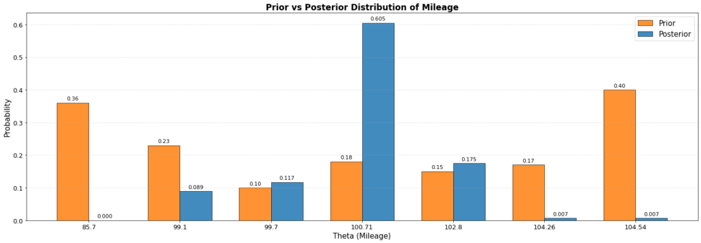
| Parameter $\theta$ | Prior | Posterior |
|---|---|---|
| 85.70 | 0.36 | 0.000 |
| 99.10 | 0.23 | 0.089 |
| 99.70 | 0.10 | 0.117 |
| 100.71 | 0.18 | 0.605 |
| 102.80 | 0.15 | 0.175 |
| 104.26 | 0.17 | 0.007 |
| 104.54 | 0.40 | 0.007 |
Interpretation
Observed value: $x = 101.25$ km/litre
1. The salesperson had strong confidence in $\theta = 104.54$ (prior = 0.40) but the observed average mileage of 101.25 indicates that $\theta = 100.71$ is far more realistic. The data updates the belief away from the prior.
2. $\theta = 100.71$ had only a modest prior (0.18) — the salesperson was not highly confident here — but the observed data strongly supported it, pushing the posterior to 0.605. Data can elevate a weakly held belief when evidence supports it.
3. $\theta = 85.70$ had a surprisingly high prior (0.36) — perhaps reflecting older, lower-mileage models. But the observed average of 101.25 gives this value a likelihood of essentially zero, so the posterior becomes 0.000. No amount of prior intuition survives when data tells a completely different story.
4. Values of $\theta$ in the neighbourhood of 99–103 receive moderate posterior support because they are close to the observed value. Prior beliefs that are already close to the truth get gently confirmed by data.
The Real Bayesian Message
The prior is the starting point — it could be an expert’s intuition, a salesperson’s experience, or a reasonable guess. The data is the ground truth from the real world. The posterior is simply what you should now believe after letting the data inform your prior. Neither dominates by force — they work together to arrive at the most honest and updated belief.
If we had only relied on the customer data alone, we would have said “the mileage is 101.25” — a single point estimate with no sense of uncertainty. But mileage varies across customers, road conditions, and driving habits. The prior captures this uncertainty across multiple plausible values. By combining informed prior beliefs with actual data, the posterior gives something richer: a probabilistic statement about which mileage values are now most credible.
This is the true power of Bayesian thinking: it does not just give you an answer — it gives you an honest picture of your uncertainty, updated by real evidence.
Your Priors Don’t Have to Be Perfect — But Your Posterior Must Be
Did you notice that the prior probabilities in Data Type III do not sum to 1?
$$0.36 + 0.23 + 0.10 + 0.18 + 0.15 + 0.17 + 0.40 = 1.59 \neq 1$$
This makes it an improper prior — technically not a valid probability distribution. Yet Bayesian inference still works here. The normalising constant $P(X)$ in the denominator of Bayes’ Theorem automatically rescales everything, and the resulting posterior is guaranteed to sum to 1 and be a proper distribution.
This is the key condition: improper priors are admissible in Bayesian inference, provided the posterior they produce is proper.
Bayesian Inference — Continuous Parameter: The Beta Distribution
Context: Hero vs Honda Mileage Dispute
The same dispute — Honda questioning Hero’s claim of 102.5 km/litre for the Splendor iSmart. iCAT tests a fixed batch of $n = 100$ bikes. Each bike either passes the mileage threshold or it does not. The observed number of bikes passing is $x = 35$.
Now instead of restricting $\theta$ to a handful of discrete candidate values, we treat it as a continuous parameter — $\theta$ can be any value in $(0, 1)$, representing the true proportion of bikes that genuinely meet the mileage claim.
Why the Beta Distribution for the Prior?
$\theta$ is a proportion — it must lie strictly between 0 and 1. The Beta distribution is defined exactly on this interval $(0, 1)$ and nowhere else. It is also highly flexible: by choosing its two shape parameters $\alpha$ and $\beta$, it can take on a wide variety of shapes — flat, bell-shaped, U-shaped, or skewed — making it a natural and honest way to express whatever prior belief an expert holds about $\theta$.
We write the prior as $\theta \sim \text{Beta}(\alpha, \beta)$.
The Data and Likelihood
Each bike independently either passes or fails. With $n = 100$ bikes tested and $x = 35$ passing, the likelihood of the observed data given any value of $\theta$ is:
$$P(X = x \mid \theta) = \binom{n}{x}\, \theta^x\, (1-\theta)^{n-x} \quad \text{with } n = 100,\ x = 35$$
The Algorithm
Step 1 — Specify the prior: Choose $\alpha$ and $\beta$ to reflect prior belief about $\theta$.
Step 2 — Observe the data: Record $n$ (batch size) and $x$ (number passing).
Step 3 — Update: Combine the prior with the likelihood using Bayes’ Theorem:
$$p(\theta \mid X) \propto P(X \mid \theta) \cdot p(\theta)$$
When the prior is $\text{Beta}(\alpha, \beta)$ and the likelihood is Binomial, this multiplication gives a clean update rule:
$$\text{Posterior} = \text{Beta}(\alpha + x,\ \beta + (n – x))$$
That is: add the number of successes to $\alpha$, and the number of failures to $\beta$.
Four Prior Shapes
The data is fixed in all four cases: $n = 100$, $x = 35$. Only the prior belief differs.
Case 1 — No Prior Knowledge: Uniform Prior Beta(1, 1)
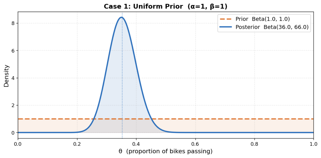
Prior: $\alpha = \beta = 1$. Every value of $\theta$ between 0 and 1 is equally plausible — we have no reason to favour any proportion over another.
Likelihood: Binomial with $n = 100$, $x = 35$.
Posterior:
$$\alpha^* = 1 + 35 = 36 \qquad \beta^* = 1 + 65 = 66 \qquad \Rightarrow \quad \text{Beta}(36,\ 66)$$
With no prior opinion, the posterior is driven entirely by the data. The posterior curve peaks very close to the observed proportion 35/100 = 0.35.
Case 2 — Extreme Uncertainty: U-shaped Prior Beta(0.5, 0.5)
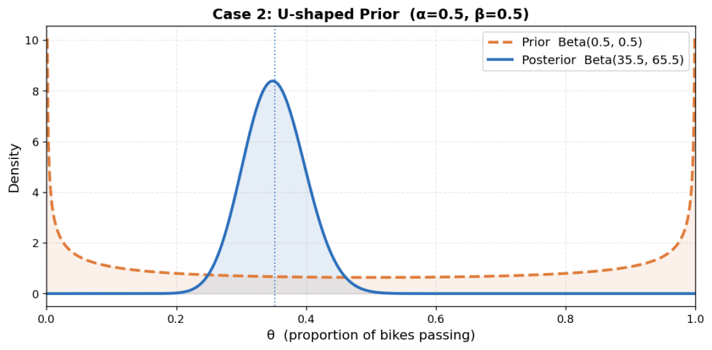
Prior: $\alpha = \beta = 0.5$. Belief that $\theta$ is near 0 or near 1 — either almost no bikes pass or almost all do. Very little mass in the middle.
Likelihood: Binomial with $n = 100$, $x = 35$.
Posterior:
$$\alpha^* = 0.5 + 35 = 35.5 \qquad \beta^* = 0.5 + 65 = 65.5 \qquad \Rightarrow \quad \text{Beta}(35.5,\ 65.5)$$
Despite the prior placing mass at the extremes, 100 observations are more than enough to override it. The posterior settles firmly around $\theta \approx 0.35$.
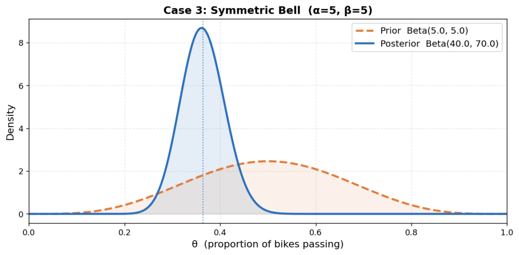
Case 3 — Centred Belief: Symmetric Bell Prior Beta(5, 5)
Prior: $\alpha = \beta = 5$. Belief that the pass rate is likely around 50%, based perhaps on prior experience with similar testing.
Likelihood: Binomial with $n = 100$, $x = 35$.
Posterior:
$$\alpha^* = 5 + 35 = 40 \qquad \beta^* = 5 + 65 = 70 \qquad \Rightarrow \quad \text{Beta}(40,\ 70)$$
The prior was pulling toward 0.50. The data pulls it back down. The posterior peaks slightly higher than Cases 1 and 2 — the prior’s influence is visible but modest.
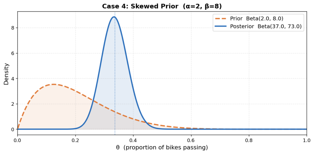
Case 4 — Pessimistic Belief: Skewed Prior Beta(2, 8)
Prior: $\alpha = 2$, $\beta = 8$. Belief that the pass rate is likely low — most mass is concentrated below 0.30.
Likelihood: Binomial with $n = 100$, $x = 35$.
Posterior:
$$\alpha^* = 2 + 35 = 37 \qquad \beta^* = 8 + 65 = 73 \qquad \Rightarrow \quad \text{Beta}(37,\ 73)$$
The prior was pessimistic but the data contradicts it. The posterior shifts noticeably upward from the prior. The prior leaves a small fingerprint — the posterior peak is slightly lower here than in the other cases — but the data dominates. A prior can slow the update; it cannot stop it.
Conclusions
Case 1 — Uniform Prior
No prior opinion means the data speaks without resistance. The posterior lands almost exactly at the observed proportion 35/100 = 0.35. This is the purest form of learning from data alone.
Case 2 — U-shaped Prior
A prior that supports or assumes “proportion of success must be near 0 or near 1” is completely overruled by 100 observations. The posterior ignores the extremes and settles around 0.35.
Case 3 — Symmetric Bell Prior
The prior believed the pass rate was around 50%. The data disagreed. The posterior is pulled downward but lands slightly above Cases 1 and 2 — the prior’s optimism leaves a small trace. This is the prior and data negotiating, with data holding the stronger hand.
Case 4 — Skewed Prior
The most opinionated prior — convinced the pass rate was low. The data pushed back hard. The posterior moves substantially away from the prior, though it peaks marginally lower than the other cases. A prior and data can help the update.
Overall Takeaway
All four posteriors converge to broadly the same region around $\theta \approx 0.33$–$0.36$, regardless of where they started. The prior shape matters most when data is scarce. When data is plentiful, it wins.