
Introduction
When we define a function in mathematics, it usually has a parameter — something that stays fixed for one particular function but can change to give a different member of the same family. This parameter helps us identify one particular member out of a whole family of similar functions.
The same idea applies to probability distributions. When we describe a random variable using its PDF or PMF, we are really picking one member out of a family of possible distributions. The parameter is what tells us which member we are talking about, and it helps us summarize and characterize the random variable we are studying.
These notes look at how probability distributions are built using such parameters, based on conditions that reflect real-world situations. Each distribution we study will have a parameter (or parameters) that define a whole family of related distributions. In practice, we usually don’t know the exact value of this parameter — instead, we estimate it from data.
This is why, when we express the probability distribution of a real-world situation, we say “a PDF” rather than “the PDF.” That is, we write $X$ follows a PDF $f(x|\theta)$, indicating that $X$ follows this distribution for some value of the parameter $\theta$. On the other hand, if $\theta$ is known, we simply say $X$ follows the PDF $f(x)$, where $\theta$ need not be specified explicitly. This distinction — between a family of distributions indexed by an unknown parameter and a single, fully specified distribution — is one of the most important bridges between mathematical thinking and statistical thinking.
For these reasons, this note uses $f(x|\theta)$ for all distributions. Here, $\theta$ refers to one or more parameters, depending on the specific case.
Bernoulli distribution
A random variable $X$ which takes two values $0$ and $1$ with probabilities $q$ and $p$ respectively is called a Bernoulli variate and is said to have a Bernoulli distribution.
These two possible values $0$ and $1$ of $X$ can be thought of as the only possible outcomes “failure” and “success” of an experiment. Therefore, $q = 1-p$ or $p+q=1$. For example, getting a head with a balanced coin (equivalently getting a tail) passing (or failing an examination), getting a defective (or non-defective) item from a lot are certain Bernoulli successes. We refer to an experiment to which the Bernoulli distribution applies as a Bernoulli trial or simply a trial and to sequences of such experiments as repeated trials.
Definition
A random variable $X$ is defined to have a Bernoulli distribution if the probability distribution of $X$ is given by
$$f_X(x|\theta) = \begin{cases} p^x(1-p)^{1-x} & x = 0, 1 \\ 0 & \text{elsewhere} \end{cases} $$
where $p$ is the parameter which satisfies $0 \leq p \leq 1$.
Here $1-p$ is often denoted by $q$ so that $p+q=1$.
Consider a random experiment tossing 3 coins simultaneously. If we extend this as a repeated trial of say 12 flips of a coin and if we want to know the probability of getting 5 heads, then our earlier approach is really cumbersome. However, we can observe that the probability of getting a head is the same for each of the 12 trials $(p = 1/2)$ and there is independence in getting the outcomes (Head or Tail). Hence, if we define “success” as getting a head, under the stated conditions we are interested in finding 5 success in 12 flips or 12 independent repeated trials.
Such repeated trials play an important role in probability and statistics. In such cases, we assume the following.
- The number of trials is fixed.
- The parameter $p$ (the probability of success) is the same for each trial.
- All the trials are independent.
There are certain random variables that arise in connection with repeated trials. One such distribution which concerns the total number of successes (5 heads in 12 flips i.e., number of successes is 5) is a Binomial distribution.
Binomial Distribution
A random variable $X$ is said to be a binomial distribution if the probability distribution of $X$ is
$$f_X(x|\theta) = \begin{cases} \displaystyle\binom{n}{x} p^x q^{n-x} & x = 0, 1, 2, \cdots n \\ 0 & \text{elsewhere} \end{cases} $$
Here $n$ and $p$ are parameters. We denote $X \sim \text{Binomial}(n, p)$ to convey that $X$ has a binomial distribution with parameters $n$ and $p$. The idea behind this probability distribution is quite natural and we find this idea now.
Assume that there are $n$ points ($n$ trials) in a straight line in which $x$ points are called as successes and remaining $n-x$ points are called failures. Using combinatorics we can select $\displaystyle\binom{n}{x}$ ways of ‘$x$’ successes. Once the success points are selected, let us apply the probability idea.
Assuming the independence and constant probability $(p)$ of success. we have the probability of getting $x$ successes (and equivalently $n-x$ failures) is $p^x(1-p)^{n-x}$ or $p^xq^{n-x}$. Hence, the probability of getting $x$ successes in $n$ trials is $\displaystyle\binom{n}{x} p^x q^{n-x}$.
Next we consider the following instance. A sequence of questions is given to a student. As soon as he records his $5^{th}$ correct answer (5 successes) the test is over and the student is declared as pass. Here we are concerning the number of trials on which the $5^{th}$ success occurs. Let us assume that answering the correct one is success event and ‘$p$’ be the probability of success. Note that the sequence must have a set of 5 questions. (so trials must be 5). Following Table 1 explains the situation.
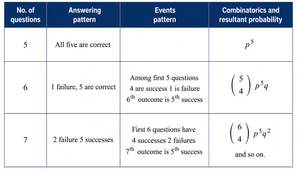
Table 1: example for Negative Binomial
Note that last column of this table assumes independence of trials and constant probability $(p)$ of success. Extending the idea in the last column, if we have $n$ questions there must be $4(5-1)$ successes and $n-5(=x)$ failures in the first $n-1$ questions and $n^{th}$ outcome must be a success (which is of course $5^{th}$ success). Hence, the last column can be generalised as $\displaystyle\binom{n-1}{4} p^5 q^{n-5}$ or $\displaystyle\binom{x+5-1}{4} p^5 q^x$. If we generalise this idea of finding the number of trials on which the $r^{th}$ success occurs, in connection with repeated Bernoulli trials, we define a random variable $X$ which is said to have a negative binomial distribution.
Negative Binomial Distribution
A random variable $X$ is said to be a negative binomial distribution if the probability distribution of $X$ is
$$f_X(x|\theta) = \begin{cases} \displaystyle\binom{x+r-1}{r-1} p^r q^x & x = 0, 1, 2, \cdots \\ 0 & \text{elsewhere} \end{cases} $$
We denote it as $X \sim \text{Negative Binomial}(x; r, p)$.
Hence negative binomial distribution represents how long one has to wait for the $r^{th}$ success, so that this random variable is offen referred to as a discrete waiting-time random variable.
If in the negative binomial distribution $r = 1$, then we get a special name for the random variable $X$. It is called the geometric distribution.
Geometric Distribution
A random variable $X$ is said to be a geometric distribution if the probability distribution of $X$ is
$$f_X(x|\theta) = \begin{cases} pq^x & x = 0, 1, 2, 3, \cdots \\ 0 & \text{elsewhere} \end{cases} $$
Here $p$ is the only parameter and we denote it as $X \sim \text{Geometric}(p)$.
One more distribution that arises from repeated trials is Poisson distribution. Specifically, when $n \to \infty$ and $p \to 0$ (equivalently $np$ is constant), the number of successes is a random variable having a poisson distribution. Hence, Poisson distribution is a limiting form of the binomial distribution, which we prove in the following result.
Binomial by Poisson
Our assumption is $n$ is very large and $p$ is very small so that their product $np$ remains constant. Let $\lambda = np$. Consider $X \sim \text{Binomial}(n, p)$, so that
$$f_X(x|\theta) = \binom{n}{x} p^x q^{n-x}$$
$$= \binom{n}{x} p^x (1-p)^{n-x} \quad x = 0, 1, 2, \cdots, n$$
Consider $\displaystyle\binom{n}{x} p^x (1-p)^{n-x}$
$$= \frac{n!}{x!(n-x)!} p^x (1-p)^{n-x}$$
$$= \frac{n(n-1)(n-2)\cdots(n-x+1)}{x!} \frac{\lambda^x}{n^x} \left(1-\frac{\lambda}{n}\right)^{n-x}$$
$$= \frac{1}{x!}\frac{n}{n}\left(\frac{n-1}{n}\right)\left(\frac{n-2}{n}\right)\cdots\left(\frac{n-x+1}{n}\right)\lambda^x\left(1-\frac{\lambda}{n}\right)^{n-x} $$
$$ = \frac{1}{x!}\left(1-\frac{1}{n}\right)\left(1-\frac{2}{n}\right)\cdots\left(1-\frac{x-1}{n}\right)\lambda^x\left(1-\frac{\lambda}{n}\right)^{n-x}$$
$$= \frac{1\left(1-\frac{1}{n}\right)\left(1-\frac{2}{n}\right)\cdots\left(1-\frac{x-1}{n}\right)}{x!}\lambda^x\left(1-\frac{\lambda}{n}\right)^n\cdot\left(1-\frac{\lambda}{n}\right)^{-x}$$
$$= 1\left(1-\frac{1}{n}\right)\left(1-\frac{2}{n}\right)\cdots\left(1-\frac{x-1}{n}\right)\left(1-\frac{\lambda}{n}\right)^{-x}\frac{\lambda^x}{x!}\left(1-\frac{\lambda}{n}\right)^n$$
As $n \to \infty$
$$\lim_{n \to \infty} f_X(x|\theta) = 1 \cdot \frac{\lambda^x}{x!} e^{-\lambda} \quad x = 0, 1, 2, \cdots$$
$$ = e^{-\lambda}\left(\frac{\lambda^x}{x!}\right) \quad \text{for } x = 0, 1, 2, \cdots. $$
Poisson Distribution
A random variable $X$ is said to be a poisson distribution if the probability distribution of $X$ is
$$ f_X(x|\theta) = \begin{cases} e^{-\lambda}\dfrac{\lambda^x}{x!} & x = 0, 1, 2, \cdots \\ 0 & \text{elsewhere} \end{cases} $$
We denote it as $X \sim \text{Poisson}(\lambda)$ since $\lambda = np$ is the only parameter.
Our next distribution is finding the number of successes in $n$ trials in the case of a sampling without replacement. Consider an example, among the $100$ applicants for a job only $60$ are actually qualified. If $4$ of the applicants are randomly selected for the next phase of interview and if we are interested in finding the probability that only $2$ of the $4$ will be qualified, then we proceed as follows.
Entire population ($100$) can be divided into qualified ($60$) and non-qualified ($40$) applicants. The number of ways in which 4 applicants can be selected from the population is $\displaystyle\binom{100}{4}$. Similarly, there are $\displaystyle\binom{60}{2}$ ways of selecting 2 qualified candidates and naturally there are $\displaystyle\binom{40}{2}$ ways of selecting the other 2 candidates.
Hence, the required probability is
$$ \frac{\displaystyle\binom{60}{2} \times \binom{40}{2}}{\displaystyle\binom{100}{4}} $$
To obtain a formula for the probability of getting $x$ successes in $n$ trials (but the sampling is without replacement) where $M$ of the $N$ (population) elements have a property (in our example, it is 60 qualified applicants). Hence, there are $\displaystyle\binom{M}{x}$ ways of choosing $x$ of the successes and $\displaystyle\binom{N-M}{n-x}$ ways of choosing $n-x$ of the $N-M$ failures. Hence out of $\displaystyle\binom{N}{n}$ ways getting $n$ elements from $N$, we have $x$ successes and $n-x$ failures. This idea is formulated so that the number of successes in trials is a random variable called the hypergeometric distribution.
Hypergeometric Distribution
A random variable $X$ is said to be a hypergeometric distribution if the probability distribution of $X$ is
$$f_X(x|\theta) =\begin{cases}\dfrac{\displaystyle\binom{M}{x}\binom{N-M}{n-x}}{\displaystyle\binom{N}{n}} & x = 0, 1, 2, \cdots, n \text{ and } x \leq M \text{ and } n-x \leq N-M \\ 0 & \text{elsewhere} \end{cases} $$
We denote it as $X \sim \text{Hypergeometric}(x; N, M, n)$.
CONTINUOUS DISTRIBUTIONS
Here several parametric families of probability density functions are presented. We shall start with a very simple distribution for a continuous random variable.
A random variable $X$ which has a constant probability over an internal $(a, b)$ where $a < b$ and $a$ and $b$ are real numbers. One can easily verify that the constant is $\left(\dfrac{1}{b-a}\right)$, hence we have the following definition.
Uniform Distribution
A random variable $X$ is said to be a uniform distribution if the probability density function of $X$ is
$$ f_X(x|\theta) = \begin{cases} \dfrac{1}{b-a} & a < x < b \\ 0 & \text{elsewhere} \end{cases} $$
We denote it by $X \sim \text{Uniform}(a, b)$ and $a$ and $b$ are the parameters.
Even though we define $X$ as being uniformly distributed over the open interval $(a, b)$ we could define it over the closed internal $[a, b]$ or over either of $(a, b]$ or $[a, b)$. One of the applications of uniform distribution we shall find in the future discussion in transformation of variables.
Uniform distribution is also called the rectangular distribution, since the shape of the density is rectangular.
Our next distribution namely normal distribution which is one of the more widely used distributions in applications of statistical methods. Variables such as length of steel rods, the score of a cricket player, and life of an electric lamp are often assumed to be random variables having normal definition. Let us define more formally now and have a detailed discussion of some of the important aspects of normal distribution.
Normal Distribution
A random variable $X$ is said to be a normal distribution if probability density function of $X$ is
$$f_X(x|\theta) = \frac{1}{\sigma\sqrt{2\pi}} e^{-\frac{(x-\mu)^2}{2\sigma^2}} \quad -\infty < x < \infty$$
We denote it by $X \sim \text{Normal}(\mu, \sigma^2)$ where $\mu$ and $\sigma^2$ are the parameters.
Note:
If the parameters are assumed as $\mu = 0$ and $\sigma = 1$, we have a special case of $X$ which is referred to as the standard normal distribution whose pdf is
$$\phi(x) = \frac{1}{\sqrt{2\pi}} e^{-\frac{x^2}{2}} \quad -\infty < x < \infty$$
Details of the special case will be studied in the subsequent chapter where as its utility in applied calculations will be discussed in this chapter itself especially in the calculation of probabilities involving $X \sim \text{Normal}(\mu, \sigma^2)$ and where we avoid (or impossible) a direct integration.
Other family of distribution that plays important roles in statistics is gamma distribution from which we get two more distributions as special cases, namely exponential distribution and chi-square distribution. The exponential distribution has been widely used as a model for lifetimes of various things such as reliability. Where as chi-square (particularly central chi-square) distribution finds a wide application and utility in testing of hypothesis that is in sampling theory, which is not listed in our discussion. But a formal definition of gamma distribution is presented here.
Gamma Distribution
A random variable $X$ is said to be a gamma distribution if its probability density function is
$$f_X(x|\theta) = \begin{cases} \dfrac{1}{\sqrt{\alpha}\beta^\alpha} x^{\alpha-1} e^{-x/\beta} & x > 0 \\ 0 & \text{elsewhere} \end{cases} $$
We denote it by $X \sim \text{Gamma}(X; \alpha, \beta)$ where $\alpha > 0$ and $\beta > 0$ are the parameters. When $\alpha$ is not a positive integer, the value of $\Gamma{\alpha}$ will have to be referred in a special table.
In gamma distribution if $\alpha = 1$ and $\beta = 1/\lambda$, we get an exponential distribution.
Exponential Distribution
A random $X$ is said to have an exponential distribution if probability density function of $X$ is.
$$f_X(x|\theta) = \begin{cases} \lambda e^{-\lambda x} & x > 0 \\ 0 & \text{elsewhere} \end{cases} $$
We denote if by $X \sim \text{Exponential}(\lambda)$ where $\lambda$ is the only parameter.
Another special case of gamma distribution namely chi-square distribution is obtained by taking $\alpha = r/2$ and $\beta = 2$.
Chi-square Distribution
A random variable $X$ is said to have a chi-square distribution, if $X$ has a probability density function
$$f_X(x|\theta) = \begin{cases} \dfrac{1}{2^{r/2} \Gamma\left(\frac{r}{2}\right)}x^{\frac{r}{2}-1}e^{-x/2} & x > 0 \\ 0 & \text{elsewhere} \end{cases} $$
We denote it by $X \sim \text{Chi-square}(r)$ and $r$ is the parameter which is referred to as the number of degrees of freedom.
Gamma and exponential distributions can be thought of as a continuous waiting time random variable so that the negative binomial and geometric distributions are the discrete analogs of these two distributions.
Now let us define another useful distribution which has a wide application in reliability theory (lifetime of an item). We call it as weibull distribution and define it as follows.
Weibull Distribution
A random variable $X$ is said to be a weibull distribution if the probability density of $X$ is
$$f_X(x|\theta) = \begin{cases} (\alpha\beta)x^{\beta-1}e^{-\alpha x^\beta} & x > 0 \\ 0 & \text{elsewhere} \end{cases} $$
We denote it by $X \sim \text{Weibull}(x; \alpha, \beta)$ where $\alpha > 0$ and $\beta > 0$ are the parameters. Observe that with $\beta = 1$, we get exponential distribution with parameter $\alpha$.
Beta distribution is our next variable whose application can be found in Bayesian inference and which is quite flexible as beta distribution can takes great variety of different shapes so that it can be used to model an experiment for which one of these shapes is appropriate.
Beta Distribution
A random variable $X$ is said to have a beta distribution if probability density function of $X$ is
$$ f_X(x|\theta) = \begin{cases} \dfrac{1}{\beta(\alpha,\beta)}x^{\alpha-1}(1-x)^{\beta-1} & 0 < x < 1 \\ 0 & \text{elsewhere} \end{cases} $$
We denote it by $X \sim \text{Beta}(x; \alpha, \beta)$ where $\alpha > 0$ and $\beta > 0$ are the parameters of a beta distribution.
If $\alpha = 1$ and $\beta = 1$, we can observe that beta distribution reduces to the uniform distribution $f_X(x|\theta) = 1$ in $(0, 1)$. This definition can also be presented using Gamma functions as
$$ f_X(x|\theta) = \begin{cases} \dfrac{\Gamma(\alpha+\beta)}{\Gamma\alpha\ \Gamma\beta}x^{\alpha-1}(1-x)^{\beta-1} & 0 < x < 1 \\ 0 & \text{elsewhere} \end{cases} $$
we have seen some important univariate special distributions in this notes. now let us know their characteristics namely mean and variance using it’s MGF (we know about MGF in previous notes). this constants play an important role in statistics. lets get to know summary and MGF of each discrete and continuous distributions one by one in the following table.
Quick Review on Distributions:
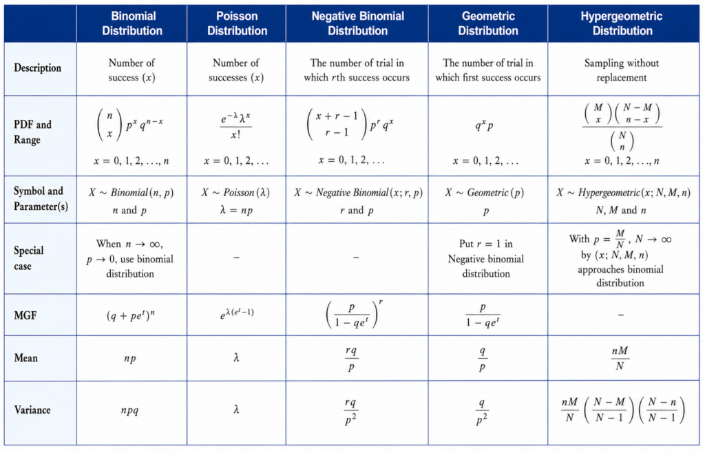
Table 2: Summary of Discrete Distributions
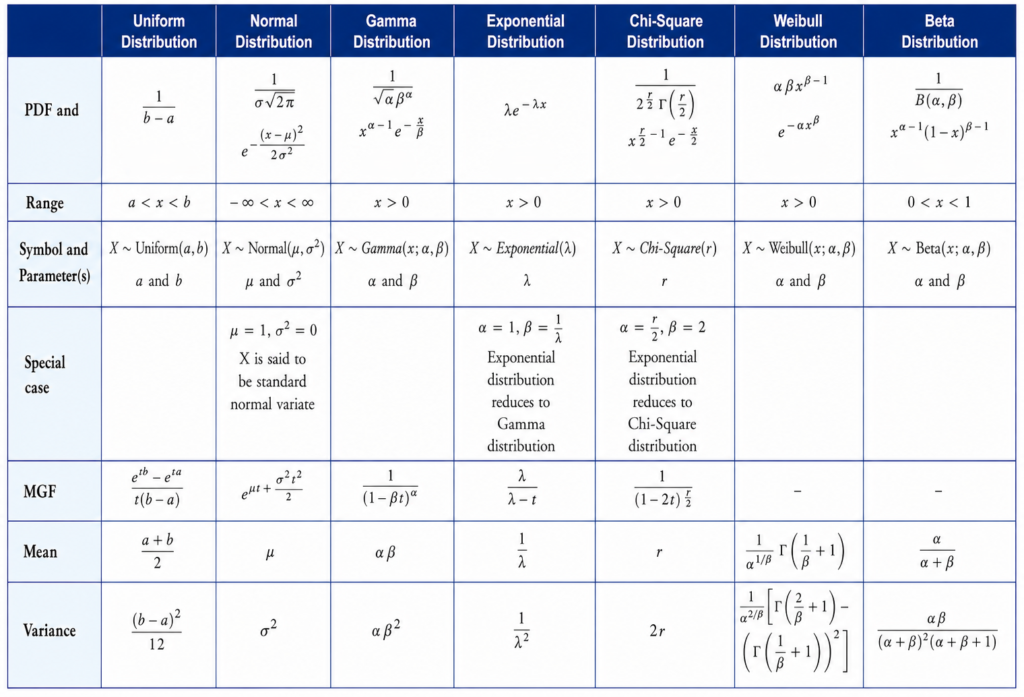
Table 3: Summary of Continuous Distributions
Properties:
- The Binomial distribution possesses the additive porperty if $p_1=p_2=p$
- Sum of independent Poisson variables is also a Poisson variables.
- The sum of two independent normal variables is also a normal variable.
- The sum of two independent gamma variables is also a gamma variable.
- If $X$ and $Y$ are independent Poisson variables the conditional distribution of $X$ given $X+Y$ is binomial.
- Let the two independent random variables $X$ and $Y$ have the geometric distribution. Then the conditional distribution of $X$ given $X+Y=n$ is uniform
- If $X$ has a geometric distribution with parameter $p$ then $p[X \ge k+t| X\ge k]=p[X \ge t]$.
- If $X$ is an exponential distribution, then $p[X \ge k+t| X\ge k]=p[X \ge t]$ for any $k$, $t>0$
Note: Properties (7) and (8) state the property of a geometric distribution and its continuous analog exponential distribution called lack of memory. In fact Property (7) states that the probability that atleast t trials are required before the first success given that there have been K successive failures is equal to the unconditional probability that atleast t trials are needed before the first success. That is, the fact that though we have already observed K successive failures will not change the probability of the number of trials required to obtain the first success. Similarly, Property (8) states that if X represents the lifetime of a given component then an old functioning component has the same lifetime distribution as a new functioning component. This property is also called as memory less property. Indeed the converse of Property (7) and Property (8) are true which we prove now. - If $X$ is a non-negative integral valued random variable and $p[X \ge k+t| X\ge k]=p[X \ge t]$ then $X$ is a geometric distribution.
- If a continuous RV $X>0$ has memory less property then $X$ has an exponential distribution.
Remark:
Mathematical thinking gives us the family of distributions through the parameter $\theta$. Statistical thinking is about finding the right value of $\theta$ from real data. This shift — from defining a family to estimating a member of it — is the bridge between mathematical thinking and statistical thinking.