Introduction
From a classical text, Mood, A. M., Graybill, F. A., & Boes, D. C. Introduction to the Theory of Statistics, we can realize the notion behind test of hypotheses “Discover some statistic (For instance, MLE) which behaves differently under two hypothesis and utilize the different behavior to design a test”; a simplest and yet most useful and intuitive technique for understanding the statistical tests. This notes provides an introduction about the statistical test of hypotheses
Suggested Reading: [CABE] Casella, G., & Berger, R. L. (2002). Statistical inference (Vol. 2). Pacific Grove, CA: Duxbury.
Suggested Reading:: [MGB] Mood, A. M., Graybill, F. A., & Boes, D. C. Introduction to the Theory of Statistics 1974 [Third Edition]. McGraw-Hill
More specifically, Chapters 7 and 8 of CABE; Chapter IX (Section 1) of MGB
Keywords:
- Likelihood function
- Estimator
- Estimate
- Maximum Likelihood Estimates (MLE)
- Statistical Hypothesis (SH)
- Simple
- Composite
- Critical region for a NRT
- Two hypotheses
- Null
- Alternative
- Two Types of error
- Type I
- Type II
- Size of error
- Power function
- Size of Test
- Level of test
Assume a parameter space in $S\subset\mathbb{R^1}$. The parameter space is divided into two disjoint sets $S_0$ and $S_1$ such that
$$S_0 \cup S_1 = S$$ and $$S_0 \cap S_1 = \phi$$
Usually this partition helps to device hypothesis (or) conversely, a hypothesis about a parameter induces such a partition.
$\Rightarrow S_0 = \{\theta \in S_0 / \textrm{Satisfy criterion of} ~H_0\}$
$S_1 = \{\theta\in S_1 / \textrm{Satisfy criterion of } ~H_1\}$
Aim is to reach a decision about $S_0$ or $S_1$
- The random experiment is to be repeated.
- A random sample from $f(x|\theta)$
- Device a rule that will help to decide between $S_0$ and $S_1$, between $H_0$ and $H_1$
- Rule means, a test of $H_0$ vs $H_1$
- Rule is based on the random sample
- Range ($\mathcal{A}$) of the random variable is used in the process.
Assume $\mathcal{A} \subset \mathbb{R^1}$ and let $A_n = \{(x_1, \cdots, x_n) / x_i \in \mathcal{A}\}$
Let $A_0 = \{(x_1, \cdots, x_n) / \textrm{Rule based on}~ (x_1,\cdots,x_n) \textrm{favours}~H_0\}$
$A_1 = \{(x_1, \cdots, x_n) / \textrm{Rule based on}~ (x_1,\cdots,x_n) \textrm{favours}~H_1\}$
$= \{(x_1, \cdots, x_n) / \textrm{Rule based on}~ (x_1,\cdots,x_n) \textrm{does not favour}~H_0\}$
Hence, $A_0 \cup A_1 = A_n$ and $A_0 \cap A_1 = \phi$; also it can be observed that $A’_0 = A_1$
$A_1=A_0’$ : Rejection Region / critical region $CR$ and $A_0$ is Acceptance Region $AR$
“Typically, a hypothesis test is specified in terms of a statistic $T(X) = W(x_1,\cdots, x_n)$ a function of the sample”
While doing this action (based on a $\underline{\textrm{rule}}$) two fold possibilities arise:
For a given process
1 $\theta \in S_0 ~~or ~~\theta\in S_1$
2 $\underline{\textrm{Rule}}$ implies $(x_1,\cdots, x_n) \in AR$ or
$(x_1,\cdots, x_n) \in CR$
These 4 combinations can be summarized as
Correct conditional events
1 $T(X)\in AR~ /~ \theta\in S_0$
2 $T(X)\in CR~ /~ \theta\in S_1$
Error conditional events
1 $T(X)\in CR ~/~ \theta\in S_0$ Type I error
2 $T(X)\in AR ~/~ \theta\in S_1$ Type II error
Size of an error
1 $\alpha = P\textrm{(Type I error)} = P(T(X)\in CR ~/~ \theta \in S_0)$
2 $\beta = P\textrm{(Type II error)} = P(T(X)\in AR ~/~ \theta \in S_1)$
Power function of a test T is the probability that $H_0$ is rejected
$$\begin{eqnarray} \pi_T(\theta) &=& \alpha ~~~~~~~~~~~~~~\textrm{whenever} ~~\theta \in S_0\\ &=& 1-\beta ~~~~~~~~\textrm{whenever} ~~\theta \in S_1 \end{eqnarray}$$
Hence,
$\pi_T(\theta) = P[T(X) \in CR]$
$=P[T(X) \in CR ~~\textrm{when}~~ \theta \in S_0 ~~\textrm{or} ~~T(X) \in CR ~~ \textrm{when} ~~\theta \in S_1 ]$
$=P[T(X) \in CR ~|~ \theta \in S_0] = \alpha$
$= P[T(X) \in CR ~|~ \theta \in S_1] = 1- P[T(X) \in AR ~|~ \theta \in S_1] = 1-\beta$
Here we use $P[A’~|~B]=1-P[A~|~B]$
Aim is to reduce these errors
- $\alpha$ and $1-\beta$ should be as low as possible
- $\alpha$ should be low, $\beta$ should be “as high as” possible
Precisely,
- $P(T(X) \in CR)$ is low when $\theta \in S_0$
- $P(T(X) \in CR)$ is high when $\theta \in S_1$
This is the desired characteristic of a test T
$i.e$ prefer a size $\alpha$ test means a test T with
$$\underset{\theta \in S_0}{\textrm{sup}}\Big[\pi_T(\theta)\Big]= \alpha ~~~~~0\leq \alpha \leq 1$$
Liberally, level $\alpha$ test has $$\underset{\theta \in S_0}{\textrm{sup}}\Big[\pi_T(\theta)\Big] \leq \alpha$$
Objective of Testing of Hypotheses
“seek a rule (based on statistic) of desired size $\alpha$”
$\textbf{Example}$
Let it be known that the outcome x of a random experiment is $N(\theta,\sigma^2)$ with $\sigma^2$ known say $\sigma^2 = 100$ so, $\theta\in (-\infty,\infty)$
Intention is to test $\theta > 75$ (a ‘natural’ or desired sentence leads to research hypothesis)
$\Rightarrow$ Parameter space is divided into $S_0:\theta \in (-\infty,75]$ and $S_1:\theta \in (75,\infty)$
Equivalently, hypotheses can be framed as $H_0=\theta \leq 75$ Vs $H_1:>75$
$\textbf{Device a test, based on CR}$
1. Test 1: Reject $H_0 \Leftrightarrow \overline {X}> 75$
2. Test 2: Reject $H_0 \Leftrightarrow \overline {X} >78$
3. Test 3: Reject $H_0 \Leftrightarrow \overline {X} >76$
In the above three tests $T(X) = \overline {X}$ (why?)
Let us assume size of the sample be
- n = 25 for Tests 1,2
- n = 100 for Test 3
$$\textbf{Computing power function:}$$
Test 1
$H_0 : \theta \leq 75$ vs $H_1 : \theta > 75$
$CR : \{(x_1,\cdots,x_{25})~/~ \overline {X} >75\}$
$$\pi_T(X) = P(T(X)\in CR) = P(\overline {X} >75)$$
when $X \sim \text{Normal}~(\theta,100)$ $\sigma^2:100$
$\bar X \sim \text{Normal}~(\theta , \frac{100}{25}) = \text{Normal}~(\theta , 4)$
Let us pick few values for $\theta$
$\theta=$ 72,73,74,75,76,77,78,79 of which $AR=$ 72,73,74,75 and $CR=$ 76,77,78,79
$\pi_T(\theta) = P(\overline {X} >75)$
$= P(\frac{\overline {X} – \theta >75}{2} > \frac{75-\theta}{2})$
$\pi_T(\theta) = P(Z > \frac{75-\theta}{2})$ where $Z\sim \text{Normal}~(0,1)$
For $~~ \theta = 72$,
$\pi_T(\theta) = P(Z > \frac{75-72}{2})$
$= P(Z>1.5) = 1-0.9332 = 0.0668$
Similarly, $\pi_T(73) = P(Z > \frac{75-73}{2})$
$= P(Z>1) = 1-0.8413 = 0.1587$
Proceeding in this way,
$\pi_T(79) = P(Z > \frac{75-79}{2})$
$= P(Z> -2 )$
$= P(Z< 2) = 0.9772$
Test 2 and 3 – Illustrated for 72
Also, $\pi_{T_2}(72) = P(\overline {X} >78)$
$\pi_{T_2}(72) = P(\frac{\overline {X} – \theta}{2}>\frac{78-72}{2}) = P(Z> 3)$
$= 1- 0.9987 =0.0013$
$\pi_{T_3}(72) = P(\frac{\overline {X} – 72}{1}>\frac{76-72}{1})$
$= P(Z> 4)$
$= 1 -0.99997 = 0.00003$
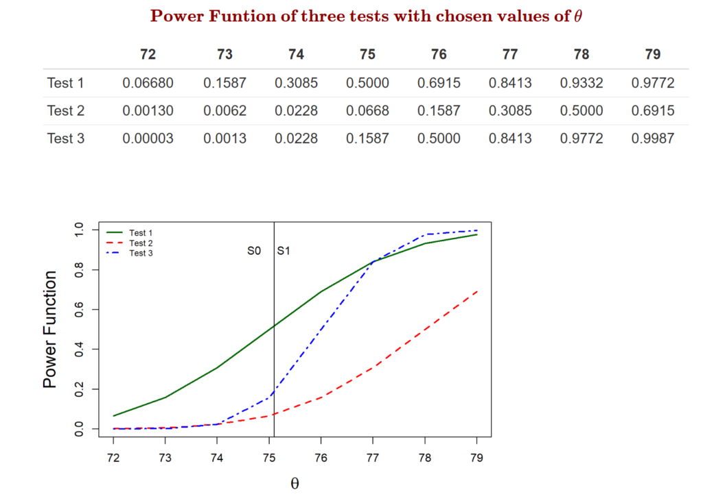
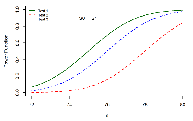
Observations
For Test 1,
- $P~[T(X) \in CR]$ is not comparatively low when $\theta \in S_0$
- Means $\alpha$ is not low in $S_0$
For Test 2,
- $P~[T(X) \in CR]$ is low when $\theta \in S_1$
- Means $1-\beta = P[T(X) \in CR ~|~ \theta \in S_1]$ is low
- So, $\beta = P[T(X) \in AR~ |~ \theta \in S_1]$ is high
For Test 3,
- $P~[T(X) \in CR]$ is low when $\theta \in S_0$
- $P~[T(X) \in CR]$ is high when $\theta \in S_1$
$\Rightarrow$ Smooth version of above exercise provides the following