
Introduction
In this note, we shall discuss Designing statistical tests for hypotheses on parameters involved in some standard distribution. This will illustrate specific models that generate data from underlying processes
Suggested Reading: [CABE] Casella, G., & Berger, R. L. (2002). Statistical inference (Vol. 2). Pacific Grove, CA: Duxbury.
Suggested Reading: [MGB] Mood, A. M., Graybill, F. A., & Boes, D. C. Introduction to the Theory of Statistics 1974. McGraw-Hill
Specifically, Chapters 7 and 8 of CABE; Chapter IX (Section 4) of MGB
Keywords:
- Likelihood function
- Estimator
- Estimate
- Maximum Likelihood Estimates (MLE)
- Sampling distribution
- Two hypotheses
- Critical region
- Two Types of error
- Size of error
- Power function
- Size of Test
- Level of test
Objectives
- Method of finding test procedure for specific models
- Understanding appropriate hypotheses
- Sampling from Normal distributions
For example,
- Process: Tossing a coin
- Distribution: Bernoulli($\theta$)
- Parameter: $\theta$
Let us remind ourselves from [MGB P425]:”A useful and intuitive technique for obtaining tests. Discover some statistic (For instance, MLE) which behaves differently under two hypothesis and utilize the different behavior to design a test”
A note on tail probabilities
An aspect regarding standard normal distribution ($Z$); however, this can be extended (may not be entirely) to other distribution based on its behavior.
We may be interested in finding a value ($Z_{\alpha}$, $0<\alpha< 1$) of Z that cuts off the right (equivalently left also) tail of a specified area $\alpha$ in the standard normal distribution.
In symbols, this can be understood as, $P(Z > Z_{\alpha})=\alpha$
Also it is easy to follow, $Z_{1-\alpha}=-Z_\alpha$ using symmetry of $Z$
A simple description
Now, $$P(Z>Z_{\alpha})=\alpha$$
$$\Rightarrow P(Z< -Z_{\alpha})=\alpha$$
$$\Rightarrow P(Z>-Z_{\alpha})=1-\alpha$$
Also by definition,
$$P(Z>Z_{1-\alpha})=1-\alpha$$
$$\Rightarrow P(Z>-Z_{\alpha})=P(Z>Z_{1-\alpha})$$
$$\Rightarrow Z_{1-\alpha}=-Z_{\alpha}$$
First, let us consider hypotheses involving the parameters $\mu$ and $\sigma^2$ of Normal distribution.
I. Normal Mean:
$\sigma^2$ is known
Let $X_1, X_2, \cdots, X_n \sim \text{Normal}~(\theta, \sigma^2)$
MLE of $\theta$ is $\overline {X}$
Z=$\frac{\overline {X} -\theta}{\frac{\sigma}{\sqrt n}}\sim \text{Normal}~(0,1)$
Use sampling distribution of $\overline {X}$
$i.e.\ \overline {X} \sim \text{Normal}~(\theta, \frac{\sigma^2}{n})$
$\textbf{Test (1):}$
$$\theta \leq \theta_0 ~~\textbf{vs} ~~ \theta>\theta_0$$
Reject $H_0$ if $\overline {X}-\theta_0 > K$ ($K > 0$ is arbitrary constant)
If the size of the test is $\alpha$ then
$\underset{\theta\le\theta_0}{\textrm{Sup}}~P\Big[\overline {X}-\theta_0>k\Big] =\alpha$
$\underset{\theta\le\theta_0}{\textrm{Sup}}~P\Big[\overline {X}-\theta>k+\theta_0-\theta\Big] =\alpha$
$\underset{\theta\le\theta_0}{\textrm{Sup}}~P\Big[\frac{\overline {X}-\theta}{\frac{\sigma}{\sqrt n}}>\frac{k}{\frac{\sigma}{\sqrt n}}+\frac{\theta_0-\theta}{\frac{\sigma}{\sqrt n}}\Big] =\alpha$
To find this supremum, we use the right tail probability of Z,
$i.e.$ When $\theta\le\theta_0$ then $\theta_0-\theta\ge0$
$\Rightarrow \frac{k}{\frac{\sigma}{\sqrt n}}+\frac{\theta_0-\theta}{\frac{\sigma}{\sqrt n}}$ increases whenever $\theta \in (-\inf,\theta_0]$, equivalently in $S_0 = \{\theta~|~\theta\le\theta_0\}$
$\Rightarrow$ right tail probability is decreasing when $\theta \in S_0$
$\Rightarrow$ Supremum occurs at $\theta=\theta_0$
Hence, $P\Big[\frac{\overline {X}-\theta}{\frac{\sigma}{\sqrt n}}>\frac{k}{\frac{\sigma}{\sqrt n}}\Big]=\alpha$
or $P\Big[\frac{\overline {X}-\theta}{\frac{\sigma}{\sqrt n}}>Z_{\alpha}\Big]=\alpha$
where $Z_\alpha=\frac{k}{\frac{\sigma}{\sqrt n}}$
$\Rightarrow k=z_\alpha\frac{\sigma}{\sqrt n}$
$\Rightarrow$ reject $H_0$ if $\overline {X}-\theta_0>z_\alpha\frac{\sigma}{\sqrt n}$
These details show how a statistical test is being designed for a desired hypothesis.
The rule is now based on
- $\sigma$
- sample size (n)
- a statistic or an estimator $T(X)=\overline {X}$
- $\alpha$, to find the right tail probability $Z_{\alpha}$
First item is assumed to be known; second and third items are related to the sample used in a situation.
What is the way to _fix_ $\alpha$?
A natural choice would be size or level of a test, which lies in $(0, ~1)$ but a lower value is preferred
$\textbf{Let us recall the Example discussed in the previous notes}$
It is known that the outcome x of a random experiment is $N(\theta,\sigma^2)$ with $\sigma^2 = 100$ and $\theta\in (-\infty,\infty)$
Desired hypothesis is to test $\theta > 75$
Parameter space is divided into $S_0:\theta \in (-\infty,75]$ and $S_1:\theta \in (75,\infty)$
Equivalently, hypotheses can be framed as $H_0:\theta \leq 75$ Vs $H_1:\theta>75$
Three tests were discussed. Now we add Test 4 using the size of the test as $\alpha=0.05$
Hence, for Test 4 we compute $k=z_\alpha\frac{\sigma}{\sqrt n}$ with
$\sigma = 10; n=25$ so that $k=3.289707$.
$\Rightarrow \theta_0+k=78.289707$ and the rule is Reject $H_0 \Leftrightarrow \overline {X} >78.289707$
Hence, our comparison becomes
1. Test 1: Reject $H_0 \iff \overline {X} > 75$
2. Test 2: Reject $H_0 \iff \overline {X} >78$
3. Test 3: Reject $H_0 \iff \overline {X} >76$
4. Test 4: Reject $H_0 \iff \overline {X} >78.289707$
Following figure helps to choose a test of size (level) $\alpha=0.05$
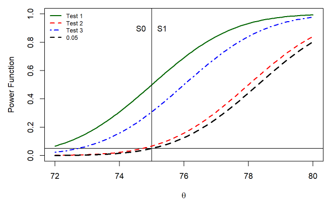
Vertical line divides the parameter space and horizontal line is the level $\alpha=0.05$
Before we proceed to further models (tests) let us understand the behaviour of a statistic (in this case, sample mean) in null and alternate space.This is to supplement the words from [MGB Pages 425-426]
“$\overline {X}$ will tend to be smaller when $H_0$ is true than when $H_0$ is false”
We do the following exercise
1. Fix a $\theta_0$;
2. Sample data from $ \text {Normal} (\theta<\theta_0,1)$ and $\text {Normal} (\theta>\theta_0,1)$ $\sigma^2$ is chosen arbitrarily as 1
3. Compute sample mean from each of the above two cases
4. Repeat this for a fixed number of times
5. Compare them in the space $S_0, S_1$
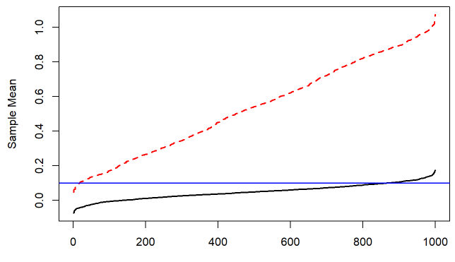
OBSERVATIONS
- Black line is the mean computed using the samples from $\text{Normal}~(\theta<\theta_0,1)$
- Red line is the mean computed using the samples from $\text{Normal}~(\theta>\theta_0,1)$
- Blue line is $\theta_0$
- It is straightforward to observe the way sample mean behaves in $S_0, S_1$
Rest of this notes describes the rule for different testing problems
$\textbf{Test (2):}$
$$\theta \geq \theta_0 ~~\textbf{vs} ~~ \theta<\theta_0$$
Reject $H_0$, if $\overline {X}$-$\theta_0<-k$, Reject if $\overline {X}<\theta_0-k$
$\Rightarrow$ if $\alpha$ is size of the test then
$\underset{(\theta\ge\theta_0)}{\textrm{Sup}}P\Big[\overline {X}-\theta_0<-k\Big] =\alpha$
$\underset{(\theta\ge\theta_0)}{\textrm{Sup}}P\Big[\overline {X}-\theta<-k+\theta_0-\theta\Big] =\alpha$
$\underset{(\theta\ge\theta_0)}{\textrm{Sup}}P\Big[\frac{\overline {X}-\theta}{\frac{\sigma}{\sqrt n}}<\frac{-k}{\frac{\sigma}{\sqrt n}}+\frac{\theta_0-\theta}{\frac{\sigma}{\sqrt n}}\Big]=\alpha$
If $\theta\ge\theta_0$ then $\theta_0-\theta\le0$
$\Rightarrow$ Supremum occurs at$\theta=\theta_0$
$P\Big[Z<\frac{-k}{\frac{\sigma}{\sqrt n}}+\frac{\theta_0-\theta}{\frac{\sigma}{\sqrt n}}\Big]=\alpha$
$\Rightarrow P\Big[Z<\frac{-k}{\frac{\sigma}{\sqrt n}}\Big]=\alpha$
$\Rightarrow 1-P\Big[Z>\frac{-k}{\frac{\sigma}{\sqrt n}}\Big]=\alpha$
$\Rightarrow P\Big[Z>\frac{-k}{\frac{\sigma}{\sqrt n}}\Big]=1-\alpha$
$\Rightarrow\frac{-k}{\frac{\sigma}{\sqrt n}}=Z_{1-\alpha}$
or$-k=Z_{1-\alpha}\frac{\sigma}{\sqrt n}$
But by symmetry,$Z_{1-\alpha}=-Z_\alpha$
$\Rightarrow$ reject $H_0$ if $\overline {X}-\theta_0<-Z_\alpha\frac{\sigma}{\sqrt n}$
$\textbf{Test (3):}$
$$\theta =\theta_0 ~~\textbf{vs} ~~ \theta\ne\theta_0$$
$\theta\neq\theta_0 \Rightarrow \theta<\theta_0$ or $\theta>\theta_0$
Reject $H_0$ if $\overline {X}-\theta_0<-k$ or $\overline {X}-\theta_0>k$
Equivalently, $|\overline {X}-\theta_0|>k$
Hence, for a test of size $\alpha$
$\underset{(\theta=\theta_0)}{\textrm{Sup}}P\Big[|\overline {X}-\theta_0|>k\Big] =\alpha$
$\underset{(\theta=\theta_0)}{\textrm{Sup}}\Bigg(P\Big[\overline {X}-\theta_0>k\Big]+P\Big[\overline {X}-\theta_0<-k\Big]\Bigg) =\alpha$
$\underset{(\theta=\theta_0)}{\textrm{Sup}}\Bigg(P\Big[Z>\frac{k}{\frac{\sigma}{\sqrt n}}+\frac{\theta_0-\theta}{\frac{\sigma}{\sqrt n}}\Big]+P\Big[Z<\frac{-k}{\frac{\sigma}{\sqrt n}}+\frac{\theta_0-\theta}{\frac{\sigma}{\sqrt n}}\Big]\Bigg) =\alpha$
$P\Big[Z>\frac{k}{\frac{\sigma}{\sqrt n}}\Big]+P\Big[Z<\frac{-k}{\frac{\sigma}{\sqrt n}}\Big]=\alpha$
$P\Big[Z>Z_1\Big]+P\Big[Z<-Z_1\Big]=\alpha$
$2P\Big[Z>Z_1\Big]=\alpha$ (By symmetry)
$Z_1=Z_{\frac{\alpha}{2}}$
Reject $H_0$ if $|\overline {X}-\theta_0|>Z_{\frac{\alpha}{2}}.\frac{\sigma}{\sqrt n}$
I. Normal Mean:
$\sigma^2$ is unknown
Use $S^2$, sample variance as an estimate of $\sigma^2$ and from the sampling distribution of $\overline {X}$ it follows that
$$\frac{\overline {X}-\theta}{\frac{S}{\sqrt n}}\sim t_{(n-1)}$$
where $t_{(n-1)}$ refers to a $t$ distribution with $n-1$ degrees of freedom
$\Rightarrow$ Three tests become,
Test 1:
$\theta\leq\theta_0$ vs $\theta>\theta_0$
Reject $H_0$ if$\overline {X} – \theta_0>t_\alpha\frac{S}{\sqrt n}$
Test 2:
$\theta\geq\theta_0$ vs $\theta<\theta_0$
Reject $H_0$ if $\overline {X} – \theta_0>t_{1-\alpha}\frac{S}{\sqrt n}$
Test 3:
$\theta=\theta_0$ vs $\theta\neq\theta_0$
Reject $H_0$ if $|\overline {X} – \theta_0|>t_{\frac{\alpha}{2}}\frac{S}{\sqrt n}$
where $t_{\alpha}$ refers the right tail probability of size $\alpha$ from a $t$ distribution with appropriate degrees of freedom
Rule of symmetry may be used appropriately
II. Comparing two means:
$X_1, X_2,\cdots,X_m \overset{iid}\sim \text{Normal}~(\theta_1,\sigma_1^2)$
$Y_1, Y_2,\cdots,Y_n \overset{iid}\sim \text{Normal}~(\theta_2,\sigma_2^2)$
X and Y are independent
Assume $\sigma_1^2$, $\sigma_2^2$ are known
$\textbf{Test (1):}$
$$\theta_1-\theta_2\leq\delta~~\textbf{vs} ~~ \theta_1-\theta_2>\delta$$
Consider
$\overline {X} = \frac{\sum X_i}{m}$ $\overline {Y} =\frac{\sum Y_i}{n}$
From the Sampling Distribution of $\overline {X}-\overline {Y}$
$$\overline {X}-\overline {Y} \sim \text {Normal}~(\theta_1-\theta_2,\frac{\sigma_1^2}{m}+\frac{\sigma_2^2}{n})$$
Hence comparing Single Normal cases,
Reject $H_0$ if $\overline {X} – \overline {Y} -\delta > Z_\alpha\sqrt{\frac{\sigma_1^2}{m}+\frac{\sigma_2^2}{n}}$
$\textbf{Test (2):}$
$$\theta_1-\theta_2\geq\delta~~\textbf{vs} ~~ \theta_1-\theta_2<\delta$$
Similarly considering the sampling distribution of $\overline {X}$-$\overline {Y}$,
Reject $H_0$ if $$\overline {X} – \overline {Y} -\delta < -Z_\alpha\sqrt{\frac{\sigma_1^2}{m}+\frac{\sigma_2^2}{n}}$$
$\textbf{Test (3):}$
$$\theta_1-\theta_2=\delta~~\textbf{vs} ~~ \theta_1-\theta_2 \ne \delta$$
Reject $H_0$ if
$\overline {X} – \overline {Y} -\delta > Z_{\frac{\alpha}{2}}\sqrt{\frac{\sigma_1^2}{m}+\frac{\sigma_2^2}{n}}$
or
$\overline {X} – \overline {Y} -\delta < -Z_{\frac{\alpha}{2}}\sqrt{\frac{\sigma_1^2}{m}+\frac{\sigma_2^2}{n}}$
or
Reject $H_0$ if $|\overline {X} – \overline {Y} -\delta| >Z_{\frac{\alpha}{2}}\sqrt{\frac{\sigma_1^2}{m}+\frac{\sigma_2^2}{n}}$
II. Comparing two means:
If $\sigma_1^2$, $\sigma_2^2$ are unknown but assume $\sigma_1^2=\sigma_2^2=\sigma^2$
Sampling distribution of $\overline {X} -\overline {Y}$ is
$\overline {X} – \overline {Y} \sim N(\theta_1-\theta_2, S_p^2)$ where
$S_p^2=\frac{(m-1)S_1^2+(n-1)S_2^2}{n+m-2}$ and
$\frac{(\overline {X}-\overline {Y})-(\theta_1-\theta_2)}{\sqrt{S_p^2 (\frac{1}{m}+\frac{1}{n})}} ~~~~\sim t_{m+n-2}$
Similar to the above three tests and related hypotheses, reject $H_0$ if
- Test 1 $\overline {X} – \overline {Y} -\delta>t_\alpha S_p \sqrt{(\frac{1}{m}+\frac{1}{n})}$
- Test 2 $\overline {X} – \overline {Y} -\delta<-t_\alpha S_p \sqrt{(\frac{1}{m}+\frac{1}{n})}=t_{1-\alpha} S_p \sqrt{(\frac{1}{m}+\frac{1}{n})}$
- Test 3 $|\overline {X} – \overline {Y} -\delta|>t_{\frac{\alpha}{2}} S_p \sqrt{(\frac{1}{m}+\frac{1}{n})}$
III. Bivariate Normal:
$(X_1,Y_1),(X_2,Y_2),\cdots,(X_n,Y_n) \sim \text{Bivariate Normal}$ and $X \sim \text{Normal}(\theta_1, \sigma_1^2)$ and
$Y\sim \text{Normal}(\theta_2, \sigma_2^2)$ are independent and let $W=X-Y$ So that $W=N(\theta_1-\theta_2, \sigma_1^2+\sigma_2^2)$
Or, $W=N(\theta,\sigma^2)$ with $\theta=\theta_1-\theta_2$ and $\sigma=\sigma_1^2+\sigma_2^2$
Hence repeating the arguments similar to inferential problems related to testing of hypotheses involving Normal mean, we have
$\hat W = \overline {X}-\overline {Y}= N(\theta,\frac{\sigma^2}{n})$ Where $\hat W = \bar W = \overline {X} – \overline {Y}$
Further if $\sigma_1^2$ and $\sigma_2^2$ are unknown, consider
$S_w^2=\frac{\sum(W_i-\bar W)^2}{n-1}$ where $W_i=X_i-Y_i$
Reject $H_0$ if
- Test 1: $\overline {W} >\theta_0+t_{\alpha,~n-1}\frac{S_w}{\sqrt n}$
- Test 2: $\overline {W} >\theta_0+t_{1-\alpha,~n-1}\frac{S_w}{\sqrt n}$
- Test 3: $|\overline {W} – \theta_0|>t_{\frac{\alpha}{2},~n-1}\frac{S_w}{\sqrt n}$
IV.Normal Variance:
$X_1,X_2,\cdots,X_n \overset{iid}\sim \text{Normal}(\mu,\sigma^2)$ where $\theta=\sigma^2$
(i) If $\mu$ is known
Consider $\hat \theta=\frac{(Xi-\mu)^2}{n}$
sampling distribution of $\hat \theta$ is obtained using the fact that $\frac{(X_i-\mu)^2}{\sigma^2} \sim \chi^2(1)$
$\frac{1}{\sigma^2}\sum (X_i-\mu)^2 \sim \chi^2(n)$
$\textbf{Test (1):}$
$$\theta\leq\theta_0 ~~\textbf{vs} ~~ \theta>\theta_0$$
Reject $H_0$ if
$\frac{\frac{\sum (xi-\mu)^2}{n}}{\theta_0}>k$ where $k>1$
Multiply and divide the numerator by $\theta$ and a simple algebra yields
$\frac{\sum (xi-\mu)^2}{\theta}>k\frac{n~\theta_0}{\theta}$
$\chi^2>k\frac{n\theta_0}{\theta}$
Now if $\alpha$ is the size of the test, then
$\underset{\theta\leq\theta_0}{\textrm{Sup}}P\Big[\chi^2>\frac{n~\theta_0}{\theta}k\Big]=\alpha$
$\Rightarrow P\Big[\chi^2>n~k\Big]=\alpha$
$n~k=\chi^2_\alpha$ $\Rightarrow k=\chi^2_\alpha.\frac{1}{n}$
Reject $H_0$ if
$\frac{\sum(x_i-\mu)^2}{n~\theta_0}>\chi^2_\alpha \frac{1}{n}$
$\Rightarrow {\sum(x_i-\mu)^2}>\theta_0\chi^2_\alpha$
$\frac{\sum(x_i-\mu)^2}{\theta_0}>\chi^2_\alpha(n)$
$\textbf{Test (2):}$
$$\theta \geq \theta_0 ~~\textbf{vs} ~~ \theta<\theta_0$$
Reject $H_0$ if
$\frac{\sum(x_i-\mu)^2}{\theta_0}<\chi_{1-\alpha}^2(n)$
$\textbf{Test (3):}$
$$\theta = \theta_0 ~~\textbf{vs} ~~ \theta \ne \theta_0$$
$\theta\neq\theta_0 \Rightarrow\theta<\theta_0$ or $\theta>\theta_0$
Reject $H_0$ if
$\sum(x_i-\mu)^2<\theta_0~k$ or $\sum(x_i-\mu)^2>\theta_0k$
If size is $\alpha$, then
$P\Big[\sum(x_i-\mu)^2>\theta_0k\Big]+P\Big[\sum(x_i-\mu)^2<\theta_0k\Big]=\alpha$
It can be noted that $\chi^2(n)$ need not be symmetry, but these two probabilities can be divided equally, so that
$P\Big[\sum(x_i-\mu)^2>\theta_0k\Big]=\frac{\alpha}{2}$ and
$P\Big[\sum(x_i-\mu)^2<\theta_0k\Big]=\frac{\alpha}{2}$
Reject $H_0$ if
$\sum(x_i-\mu)^2>\theta_0\chi^2_{\frac{\alpha}{2}}$ or
$\sum(x_i-\mu)^2>\theta_0\chi^2_{1-\frac{\alpha}{2}}$
(ii) If $\mu$ is unknown
Consider $S^2=\frac{\sum(xi-\overline {X})^2}{n-1}$
and $\frac{(n-1)s^2}{\sigma^2}=\chi^2_{n-1}$
Reject $H_0$ if
1. Test 1: $\sum(x_i-\overline {X})^2>\theta_0 \chi^2_{\alpha}(n-1)$
2. Test 2: $\sum(x_i-\overline {X})^2<\theta_0 \chi^2_{1-\alpha}(n-1)$
3. Test 3: $\sum(x_i-\overline {X})^2>\theta_0 \chi_{\frac{\alpha}{2}}^2(n-1)$ or
$\sum(x_i-\overline {X})^2<\theta_0 \chi_{1-\frac{\alpha}{2}}^2(n-1)$
V. Bivariate Normal:
Equality of Variance:
$X_1,\cdots,X_m \sim \text{Normal}(\mu_1,\sigma_1^2)$ and
$Y_1,\cdots,Y_n\sim \text{Normal}(\mu_2,\sigma_2^2)$
(i) If $\mu_1$ & $\mu_2$ are known
$\textbf{Test (1):}$
$$\sigma_1^2\leq\sigma_2^2 ~~\textbf{vs} ~~ \sigma_1^2>\sigma_2^2$$
$\frac{\sum(X_i-\mu_1)^2}{\sigma_1^2}\sim\chi^2(m)$ and
$\frac{\sum(Y_i-\mu_2)^2}{\sigma_2^2}\sim\chi^2(n)$
We can use the following result
If $U \sim \chi^2(p)$, $V \sim \chi^2(q)$ and $U$, $V$ independent then $\frac{\frac{U}{p}}{\frac{V}{q}}\sim F_{p,q}$
$\Rightarrow$ $\frac{\frac{\sum(X_i-\mu_1)^2}{\sigma_1^2}}{\frac{\sum(Y_i-\mu_2)^2}{\sigma_2^2}}\sim F_{m,n}$
We can use the ML estimate of $\sigma^2_{1}$ and $\sigma^2_{2}$
Reject $H_0$ if
$\frac{\frac{1}{m}\sum (x_i-\mu_1)^2}{\frac{1}{n}\sum (y_i-\mu_2)^2}>k$
or
$\frac{\frac{\sigma_1^2}{m}\frac{\sum(x_i-\mu_1)^2}{\sigma_1^2}}{\frac{\sigma^2}{n}\frac{\sum (y_i-\mu_2)^2}{\sigma_2^2}}>k$
$\Rightarrow \frac{\frac{1}{m}\frac{\sum(x_i-\mu_1)^2}{\sigma_1^2}}{\frac{1}{n}\frac{\sum (y_i-\mu_2)^2}{\sigma_2^2}}>k\frac{\sigma_2^2}{\sigma_1^2}$
If $\alpha$ is the size of the test, then
$\underset{\sigma_1^2\leq\sigma_2^2}{\textrm{SUP}}P\Big[F>k\frac{\sigma_2^2}{\sigma_1^2}\Big]=\alpha$
$\Rightarrow k=F_{m,n,\alpha}$
Reject $H_0$ if
$\frac{\sum(x_i-\mu_1)^2}{\sum(y_i-\mu)^2}>F_{m,n,\alpha}\frac{m}{n}$
$\textbf{Test (2):}$
$$\sigma_1^2\geq\sigma_2^2~~\textbf{vs} ~~\sigma_1^2<\sigma_2^2$$
Similar to Test 1 of Equality of variance,
Reject $H_0$ if
$\frac{\sum(x_i-\mu_1)^2}{\sum(y_i-\mu_2)^2}<\frac{m}{n}F_{m,n,(1-\alpha)}$
$\textbf{Test (3):}$
$$\sigma_1^2=\sigma_2^2 ~~\textbf{vs} ~~ \sigma_1^2\neq\sigma_2^2$$
Reject $H_0$ if
$\frac{\sum(x_i-\mu_1)^2}{\sum(y_i-\mu_2)^2}>\frac{m}{n}F_{m,n,\frac{\alpha}{2}}$ or
$<\frac{m}{n}F_{m,n,1-\frac{\alpha}{2}}$
(ii) If $\mu_1$, $\mu_2$ are unknown
Again, We use the following result
If $U \sim \chi^2(p)$, $V \sim \chi^2(q)$ and $U$, $V$ independent then $\frac{\frac{U}{p}}{\frac{V}{q}}\sim F_{p,q}$
$(m-1)\frac{S_1^2}{\sigma_1^2}\sim\chi^2(m-1)$
$(n-1)\frac{S_2^2}{\sigma_2^2}\sim\chi^2(n-1)$
$\frac{\frac{(m-1)\frac{S_1^2}{\sigma_1^2}}{(m-1)}}{\frac{(n-1)\frac{S_2^2}{\sigma_2^2}}{n-1}}=F_{m-1,n-1}$
$\Rightarrow \frac{\frac{S_1^2}{\sigma_1^2}}{\frac{S_2^2}{\sigma_2^2}}\sim F_{m-1,n-1}$
$\textbf{Test (1):}$
Reject $H_0$, if
$\frac{S_1^2}{S_2^2}>k$
$\frac{{\sigma_1^2}\frac{S_1^2}{\sigma_1^2}}{{\sigma_2^2}\frac{S_2^2}{\sigma_2^2}}>k$
$\frac{\frac{S_1^2}{\sigma_1^2}}{\frac{S_2^2}{\sigma_2^2}}>\frac{\sigma_2^2}{\sigma_1^2}k$
For size $\alpha$,
$\underset{\sigma_1^2\leq \sigma_2^2}{\textrm{SUP}}P\Big[F>k\frac{\sigma_2^2}{\sigma_1^2}\Big]=\alpha$
$k=F_{m-1,n-1,\alpha}$
Reject $H_0$ if
$\frac{S_1^2}{S_2^2}>F_{m-1,n-1,\alpha}$
Similarly other two tests can be designed
Reject $H_0$ if
- Test 2 $\frac{S_1^2}{S_2^2}< F_{m-1,n-1,1-\alpha}$
- Test 3 $\frac{S_1^2}{S_2^2}>F_{m-1,n-1,\frac{\alpha}{2}}$ (or)
- $\frac{S_1^2}{S_2^2}< F_{m-1,n-1,1-\frac{\alpha}{2}}$
A note on F-Distribution
Let $P(F_{m,n}> F_\alpha)=\alpha$
Now, $P(F_{m,n}>F_{1-\alpha})=1-\alpha$
$\Rightarrow1-P(F_{m,n}>F_{1-\alpha})=\alpha$
$\Rightarrow P(F_{m,n}\leq F_{1-\alpha})=\alpha$
$P(\frac{1}{F_{m,n}}>\frac{1}{F_{1-\alpha}})=\alpha$
$P(F_{n,m}>\frac{1}{F_{1-\alpha}})=\alpha$
$\Rightarrow F_{m,n,\alpha}=\frac{1}{F_{n,m,1-\alpha}}$ or
$F_{m,n,1-\alpha}=\frac{1}{F_{n,m,\alpha}}$
VI. Testing many means:
Let $X_{ij} \sim \text{Normal}~(\theta_i,\sigma^2)$ $j = 1,2,\cdots,n_i$; $i=1,2,\cdots,k$
Hypothesis is
$H_0:\theta_1=\theta_2=\cdots=\theta_k$ vs $H_A:\theta_r\neq\theta_t$ atlest one pair $r,t$ where
$1\leq r < t \leq k$
Instead of the ‘trick’ of choosing an estimator we apply Likelihood Ratio Test (LRT)
Reject $H_0$ if
$\frac{[MaxL(\theta|X)]_{H_0}}{[MaxL(\theta|X)]_{H_1}}< k$
Consider the Likelihood function for each i, $X_{ij}\sim \text {Normal}(\theta_i,\sigma^2)$
$L(\theta_i|X)=\prod_{j=1}^{n_i}(\frac{1}{\sigma\sqrt{2\pi}})\exp\Big[\frac{-1}{2\sigma^2}(x_{ij}-\theta_i)^2\Big]$ where $i=1,2,\cdots,k$
$L(\theta|X)=\prod_{i=1}^{k}\prod_{j=1}^{n_i}(\frac{1}{\sigma\sqrt{2\pi}})\exp\Big[\frac{-1}{2\sigma^2}(x_{ij}-\theta_i)^2\Big]$
$=\Big[\frac{1}{\sigma\sqrt{2\pi}}\Big]^n\exp\Big[\frac{-1}{2\sigma^2}\sum_{i=1}^{k}\sum_{j=1}^{n_i}(x_{ij}-\theta_i)^2\Big]$
where $n=\sum n_i$
Parameters are $\theta_1 \cdots \theta_k,\sigma^2$
under $H_0$, MLE is
$\hat \theta = \overline {X} =\frac{\sum\sum x_{ij}}{n}$ and
$\hat \sigma^2=\frac{1}{n}\sum\sum (x_{ij}-\overline {X})^2$
under $H_A$, MLE is
$\hat \theta_i = \overline {X}_i=\frac{\sum_{j-1}^{n_i} x_{ij}}{n}$
$\hat \sigma^2=\frac{1}{n}\sum\sum (x_{ij}-\overline {X})^2$
Under $H_0$, $L\Big[\theta|X\Big]$ is
$\Big[\frac{1}{n}\sum\sum (x_{ij}-\overline {X})^2 2\pi\Big]^{\frac{-n}{2}} \exp\Big[\frac{-n}{2}\Big]………………………..$(1)
Under $H_A$, $L\Big[\theta|X\Big]$ is
$\Big[\frac{1}{n}\sum\sum (x_{ij}-\overline {X}_i)^2 2\pi\Big]^{\frac{-n}{2}} \exp\Big[\frac{-n}{2}\Big]………………………..$(2)
LRT $\Rightarrow$ Reject $H_0$ if $\frac{(1)}{(2)}< k$
$\Rightarrow$ $\frac{{\Big[\sum\sum(x_{ij}-\overline {X})^2\Big]}^{\frac{-n}{2}}}{{\Big[\sum\sum(x_{ij}-\overline {X}_i)^2\Big]}^{\frac{-n}{2}}}< k………………………..$(3)
Now,
$\sum\sum(x_{ij}-\overline {X})^2=\sum\sum(x_{ij}-\overline {X}_i+\overline {X}_i-\overline {X})$
$=\sum_{i=1}^{k}\sum_{j=1}^{n_i}(x_{ij}-\overline {X}_i)^2+\sum_{i=1}^{k}\sum_{j=1}^{n_i}(X_{i}-\overline {X}_i)^2 +0$ $\because \sum\sum(x_{ij}-\overline {X}_i)=0$
$=\sum_{i=1}^{k}\sum_{j=1}^{n_i}(x_{ij}-\overline {X}_i)^2+\sum_{i=1}^{k}n_i(\overline {X}_i-\overline {X})^2$
From (3) it follows that
Reject $H_0$ if
$\Big[1+\frac{\sum n_i(\overline {X}_i-\overline {X})^2}{\sum\sum(x_{ij}-\overline {X}_i)^2}\Big]^{\frac{-n}{2}}< k$
$\Big[1+\frac{(k-1)\frac{1}{k-1}\sum n_i(\overline {X}_i-\overline {X})^2}{(n-k)\frac{1}{n-k}\sum\sum(x_{ij}-\overline {X}_i)^2}\Big]^{\frac{-n}{2}}< k$
This follows from the following fac
Numerator has k items and degress of freedom (DF) k-1;whereas,in the denominator DF for each term is $n_i$-1 DF. Hence DF is $\sum n_i$-k=n-k
$\Rightarrow$ Variance or F-ratio is
$r=\frac{\frac{1}{k-1}\sum n_i(\overline {X}_i-\overline {X})^2}{\frac{1}{n-k}\sum\sum(x_{ij}-\overline {X}_i)^2}>c$,for some $c>0$
$\Rightarrow$ the constant $c>0$ is determined so that the test will have size $\alpha$
$\Rightarrow \underset{\theta =\theta_0}{\textrm{sup}}P\Big[R\geq c/\textrm{under}~ H_0\Big]=\alpha$
$P\Big[R\geq c/\textrm{under}~ H_0\Big]=\alpha$
Now numerator of r $\Rightarrow$
$\frac{\frac{\sum n_i(\overline {X}_i-\overline {X})^2}{k-1}}{\sigma^2}\sim \chi^2_{(k-1)}$
And denominator of r $\Rightarrow$
$\frac{\frac{\sum\sum(\overline {X}_{ij}-\overline {X})^2}{n-k}}{\sigma^2}=\chi^2_{(n-k)}$
Also, $\overline {X}_i$ is independent of $\sum(x_{ij}-\overline {X}_i)^2$ and hence $R\sim F_{(k-1,n-k)}$ under $H_0$
$\Rightarrow P\Big[R \geq c\Big]=\alpha$
$\Rightarrow c=F_\alpha$
Working (computing) procedure of the above test is based on the following steps
1. For each of the k Samples find their means
$\overline {X}_1=\frac{\sum_j x_{1j}}{n_1}$
$\overline {X}_2=\frac{\sum_j x_{2j}}{n_2}$ etc
$\overline {X}_k=\frac{\sum_j x_{kj}}{n_k}$
2. Compute $\overline {X} = \frac{\sum_j\sum_i x_{ij}}{n}$ where $n=n_1+~n_2+\cdots+~n_k$
3. Find Sum of Squares Within samples – SSW:
$\sum_{i=1}^{k}\sum_{j=1}^{n_i}(x_{ij}-\overline {X}_i)^2$
(ie) first find $\sum (x_{ij}-\overline {X}_i)^2$ for each $i$ and add over $i=1,2,\cdots,k$
4. Find Sum of Squares Between samples – SSB:
$\sum_{i=1}^{k}n_i~(\overline {X}_i-\overline {X})^2$
5. Find Mean Square Error: Between (MSB) and Within (MSW)
$\textrm{MSB:} \frac{\textrm{SSB}}{\textrm{DF}}=\frac{\textrm{SSB}}{k-1}$
$\textrm{MSW:} \frac{\textrm{SSW}}{\textrm{DF}}=\frac{\textrm{SSW}}{n-K}$
$\Rightarrow F$ ratio = $\frac{\textrm{MSB}}{\textrm{MSW}}\sim F_{k-1,n-k}$
Reject $H_0$ if F>$F_{\alpha}$
where $F_\alpha$ is such that $P\Big[F>F_k\Big]=\alpha$