Introduction
A large and practically important class of functions — the elementary functions — can be built from these five basic function types under five operations (+, −, ×, ÷, ∘). Many, though not all, real-world phenomena and probability distributions can be approximated or exactly described using this class.
In mathematics, when we refer to a parameter in a functional form — for example, x² + y² = r² — it generates a family of circles, and changing r produces different members of that family. Such parameters are useful for describing characteristics of the function through operations like addition, multiplication, or exponentiation. Geometrically, this can be understood as translation, expansion or contraction, or even a change in the underlying shape.
Conventional notations
Following is a broad way of understanding various symbols used to represent random variables and distributions. However, this can be modified in a specific context; for more details, please refer
- Variables: Upper case Latin alphabets $X, Y, Z$ (preferably last 6 letters)
- Unknown Value of a variable: Lower case Latin alphabets $x, y, z$ (preferably last 6 letters)
- Constants: Lower case Latin alphabets $a, b, c$
- Transformations: Lower case Latin alphabets $a,b,c,k,l, m, n$ (except possibly the last 5 letters) or Lower case Greek alphabets $\alpha, \beta, \gamma$
- Also, Upper case Latin alphabets are used to list more variables $X_1, X_2, \cdots\cdots X_n$ and values of corresponding variables are denoted using lower case Latin alphabets $x_1, x_2, \cdots\cdots x_n$ are used.
- In the previous point, we could note another aspect called index to specify the number of variables. Lower Latin alphabets are used for index such as $i=1,2,3\cdots\cdots N$ or $j=1,2,3\cdots\cdots n$
Functional Forms
Symbolically, a function is written as:
$$y = f(x)$$
where $x$ is the independent variable and $y$ is the dependent variable; $f$ represents the relation between them. These are arbitrary symbols and can be replaced contextually — e.g., $u = g(t)$, $\theta = f_1(r)$, etc.
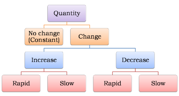
A relation between variables explains the way one influences the other — specifically, how the dependent variable changes (or does not change) when the independent variable changes.
Figure 1: Five possible forms of change in a quantity
The Five Functional Forms
The five types differ mainly in direction (growth / decay) and speed of change. In all that follows, $x$ is the independent variable, $k$ is a constant, and $a, b, c$ are parameters — unknown constants that define a family of functions.
1. Constant Function
$$f(x) = k$$
The dependent variable does not change regardless of $x$. This is a special case of the power function with exponent zero: $f(x) = ax^0 = a$.
2. Power Function
$$f(x) = ax^b + c \quad \text{(except possibly at } x = 0\text{)}$$
- Base is a variable ($x$); Exponent is a constant ($b$)
When $b = 1$, this is a linear function (straight line) — the rate of change of $y$ with respect to $x$ is constant. When $b > 2$, the function is non-linear (curvilinear) and grows faster than a straight line, especially beyond $x \approx 7.5$.
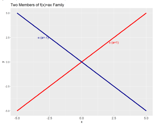
The parameters $a, b, c$ define a family. For example, $ax + c\ (b=1)$ is a family of straight lines; setting $c = 0$ restricts it to lines through the origin. Both $f(x) = x$ and $f(x) = -x$ are members of this family, differing only in direction.
Figure 2: Family of linear functions — same form, different parameter values
3. Exponential Function
$$f(x) = k^x \quad \text{with } k > 0$$
- Base is a constant ($k$); Exponent is a variable ($x$)
The exponential function grows dramatically faster than both linear and power functions — especially beyond $x \approx 5$. The most scientifically important special case is $k = e$, known as Euler’s number.
Euler’s Number $e$ — The Heart of Exponential Growth
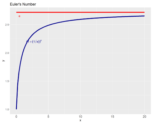
Euler’s number $e$ is one of the most fundamental constants in mathematics and statistics. It is not defined arbitrarily — it arises naturally as the limiting value of:
$$f(x) = \left(1 + \frac{1}{x}\right)^x, \quad x > 0$$
As $x \to \infty$, this expression converges to:
$$e \approx 2.71828\ldots$$
It lies between 2 and 3, and is irrational and transcendental — its decimal expansion never terminates or repeats.
Figure 3: The function (1 + 1/x)^x converges to Euler’s number e ≈ 2.718 as x increases
Why $e$ is indispensable in modeling:
- It is the base of the natural logarithm: $\ln(x) = \log_e x$
- It governs all continuous growth and decay processes
- It is the foundation of the exponential family of distributions — Normal, Poisson, Gamma, Beta, and many others all belong to this family
- It appears in Maximum Likelihood Estimation (MLE) through the log-likelihood function $\ln L(\theta)$
- It makes calculus clean: the derivative of $e^x$ is $e^x$ itself — a unique and powerful property
4. Logarithmic Function
$$f(x) = \log_m x \quad \text{where } m > 0 \text{ is the base}$$
- Common logarithm: $m = 10$
- Natural logarithm: $m = e$ (Euler’s number)
- Binary logarithm: $m = 2$
The logarithmic function is the inverse of the exponential, making it equally essential in modeling:
- Transforms multiplicative relationships into additive ones
- Central to log-likelihood in statistical estimation
- Used for linearising skewed or curved data before fitting models
Key insight: Exponential and logarithmic forms — both deeply connected through Euler’s number $e \approx 2.718$ — are the backbone of distribution theory.
5. Trigonometric (Circular) Functions
Functions such as $\sin(x)$, $\cos(x)$, $\tan(x)$ are periodic functions defined on circular geometry. Most useful for modeling cyclical or seasonal patterns in time series analysis, signal processing, and circular statistics.
Visual Representations
In this section, we provide some graphical form of above functional representations. Also, the role of transformations could be visually understood
Additive Transformation
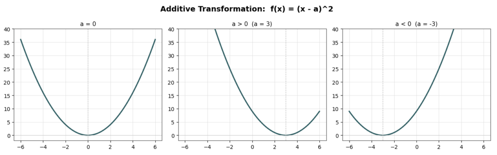
The major need for a Additive transformation is to denote the shift or (geometrically,translation) moving to left or right (below or above) of a fixed number in the range $\mathscr{A}_x$ of $X$. Such fixed number may be zero or any specific value such as mean of the random variable $X$. Usually, it is in the form of $f(x-a)$
For the first curve $x^2$, zero is the origin or $a$; in other two curves, origin is shifted by three units on either side of zero.
Multiplicative Transformation
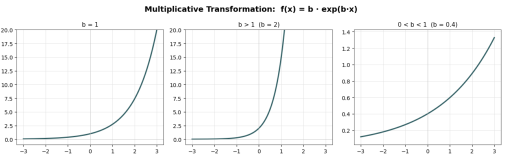
Secondly, Multiplicative transformation is useful in learning about the dispersion or spread of a distribution; larger the Multiplicative transformation, the more spread out the distribution. Its usual form is $f(\frac{x}{b})$.
For different values of Multiplicative transformation $b$ in $e^{\frac{x}{b}}$ from -3 to 3
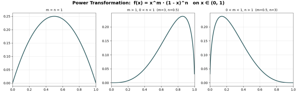
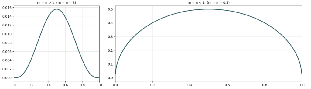
Power Transformation
Thirdly, Power transformations are to represent various Powers of a function from the same family. Its general form could be $x^m$ with suitable values for $m$
Derived from the Five Elementary Functions
Rational Functions
A rational function is a ratio of two power functions (polynomials):
$$f(x) = \frac{P(x)}{Q(x)} = \frac{a_n x^n + \cdots + a_1 x + a_0}{b_m x^m + \cdots + b_1 x + b_0}, \quad Q(x) \neq 0$$
Derived from: Power function (numerator and denominator are both polynomials)
The key condition is that the denominator $Q(x) \neq 0$ — wherever $Q(x) = 0$, the function is undefined.
Examples
$$f(x) = \frac{1}{x}, \quad x \neq 0$$
$$f(x) = \frac{x^2 + 1}{x – 2}, \quad x \neq 2$$
Hyperbolic Functions
Hyperbolic functions are defined using the exponential function — making them direct descendants of the exponential base form:
$$\sinh(x) = \frac{e^x – e^{-x}}{2} \qquad \cosh(x) = \frac{e^x + e^{-x}}{2}$$
$$\tanh(x) = \frac{\sinh(x)}{\cosh(x)} = \frac{e^x – e^{-x}}{e^x + e^{-x}}$$
And the reciprocal hyperbolic forms:
$$\text{csch}(x) = \frac{1}{\sinh x}, \quad \text{sech}(x) = \frac{1}{\cosh x}, \quad \coth(x) = \frac{1}{\tanh x}$$
Derived from: Exponential base form $e^x$ (and $e^{-x}$)
Transcendental Functions
Functions that cannot be expressed as a finite combination of algebraic operations on polynomials. They “transcend” algebra.
Derived from: Exponential, logarithmic, and trigonometric base forms.
Exponential–Logarithmic: $e^x$, $\ln x$, $a^x$, $\log_a x$
Trigonometric: $\sin x$, $\cos x$, $\tan x$
Hyperbolic: $\sinh x$, $\cosh x$, $\tanh x$
Inverse Hyperbolic Functions
Since hyperbolic functions are derived from exponentials, their inverses can be expressed as logarithms:
$$\sinh^{-1}(x) = \ln\left(x + \sqrt{x^2 + 1}\right)$$
$$\cosh^{-1}(x) = \ln\left(x + \sqrt{x^2 – 1}\right), \quad x \geq 1$$
$$\tanh^{-1}(x) = \frac{1}{2}\ln\left(\frac{1+x}{1-x}\right), \quad |x| < 1$$
Inverse Functions — Reversing the Relationship
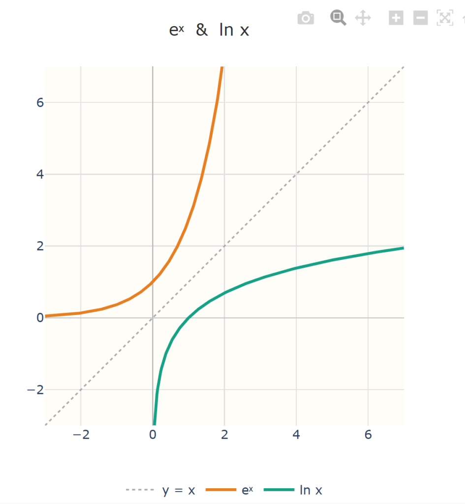
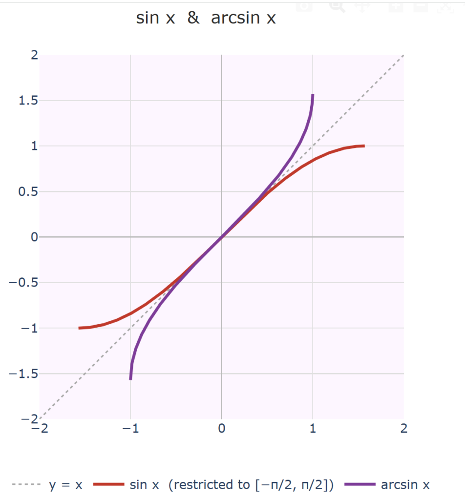
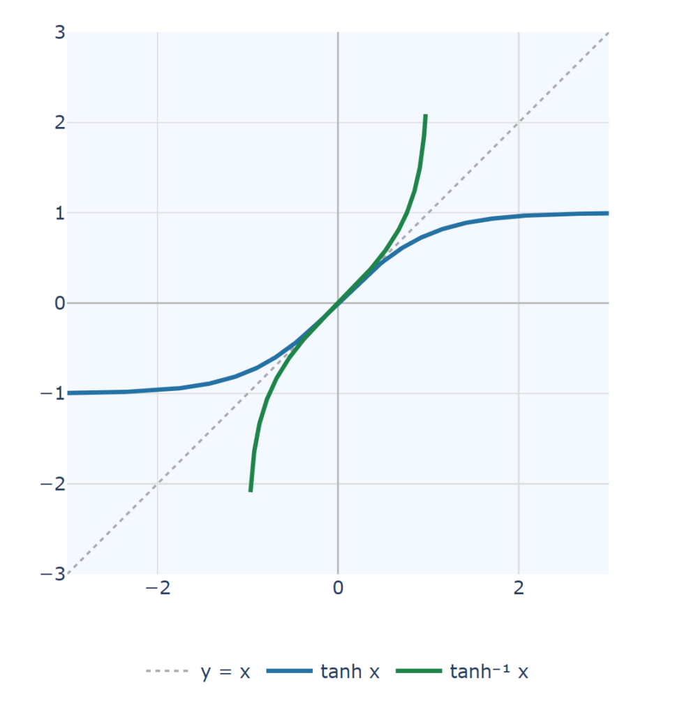
A function f(x) maps an independent variable x to a dependent variable y. Its inverse f⁻¹ simply reverses this — where f takes x to y, the inverse takes y back to x. Every input-output pair (x, y) of f becomes the pair (y, x) in f⁻¹.
This swap has a direct geometric reading: plotting f⁻¹ is the same as plotting f with its axes exchanged, which is precisely what a reflection across the line y = x achieves. The line y = x helps see this — a point (a, b) on f and its mirror (b, a) on f⁻¹ are always equidistant from it.
The plots illustrate this for three function pairs drawn from the exponential and trigonometric base forms: eˣ with ln x, sin x with arcsin x, and tanh x with tanh⁻¹ x. In each case, the inverse exists because the original function is one-to-one over its domain — a necessary condition for the reversal to be well-defined.