
For theoretical developments, refer
In Python, linear models can be directly implemented using libraries such as statsmodels (via statsmodels.formula.api.ols) or scikit-learn (via sklearn.linear_model.LinearRegression). In statsmodels, the set of arguments/inputs include a formula connecting the response variable (numeric) and the set of predictors, of the form $ y \sim x_1 + x_2 + \cdots x_k$. The intercept or constant term is directly added to the model matrix by default (unless suppressed with -1 in the formula).
Further details about ols() can be found in the official reference pages.
From the theoretical reference mentioned, it can be observed that the OLS solution is basically a “closed form” solution and all the computations are arithmetic and matrix operations. Hence, implementing it natively — without relying on statsmodels or scikit-learn — using only numpy for the underlying matrix algebra (@, .T, np.linalg.inv, np.linalg.det) may not be a very difficult task; here, is one such reproducible coding implementation.
import numpy as np
from scipy import stats

# -------------------------------------------------
#An artificial data set
x1 = [37, 45, 38, 42, 31]
x2 = [4, 0, 5, 2, 4]
y1 = [71, 66, 75, 70, 65]      # Response variable


# -------------------------------------------------
# Necessary inputs
k   = 2                    # No. of regressors
n   = len(x1)               # No. of data points
p   = k + 1                 # No. of parameters (incl. intercept)
alp = 0.05                  # Alpha for (1-alpha)*100% CI

# -------------------------------------------------
# Build model matrix X = [1, x1, x2]
xd = np.array([x1, x2]).T          # n x k matrix of predictors
xo = np.ones((n, 1))               # column of 1's
x  = np.hstack((xo, xd))           # n x p design matrix
y  = np.array(y1).reshape(n, 1)    # n x 1 response vector

m = x.T @ x                        # X'X
d = np.linalg.det(m)               # determinant of X'X

# -------------------------------------------------
# Check singularity
if d != 0:
    print("Matrix X'X is NOT singular")
else:
    print("Matrix X'X is singular")

# -------------------------------------------------
# mi = inverse of X'X
mi = np.linalg.inv(m)

# -------------------------------------------------
# OLS beta coefficients:  beta = (X'X)^-1 X'y
betao = mi @ x.T @ y

# -------------------------------------------------
# Residual sum of squares, MSE, covariance of betas
SSRes = (y.T @ y - betao.T @ x.T @ x @ betao)[0, 0]
MSRes = SSRes / (n - k - 1)
covao = MSRes * mi

print("\nSSRes, MSRes:")
print(SSRes, MSRes)

# -------------------------------------------------
# Regression sum of squares
SSR = (betao.T @ x.T @ y)[0, 0] - (sum(y1) ** 2) / n
MSR = SSR / k
SST = SSRes + SSR

# -------------------------------------------------
# Overall adequacy (F-test)
F_O      = MSR / MSRes
pval_F_O = 1 - stats.f.cdf(F_O, k, n - p)
Rsquare_O    = SSR / (SSR + SSRes)
AdjRsquare_O = 1 - ((SSRes / (n - k - 1)) / ((SSR + SSRes) / (n - 1)))

# -------------------------------------------------
# Standard errors of coefficients (diagonal of covao)
dia_elt = np.zeros(p)
for i in range(p):
    dia_elt[i] = np.sqrt(covao[i, i])

# t-statistics and p-values for each coefficient
calc_t = betao.flatten() / dia_elt
pval_O = 2 * (1 - stats.t.cdf(np.abs(calc_t), df=n - k - 1))

# -------------------------------------------------
# Confidence intervals for beta estimates
tval = abs(stats.t.ppf(alp / 2, n - p))
LL = np.zeros(p)
UL = np.zeros(p)
for i in range(p):
    LL[i] = betao[i, 0] - tval * dia_elt[i]
    UL[i] = betao[i, 0] + tval * dia_elt[i]

# -------------------------------------------------
# Unit-length scaling -> standardized regression coefficients
dif = np.zeros((n, k))
ssu = np.zeros(k)
w   = np.zeros((n, k))

for h in range(k):
    col_mean = np.mean(xd[:, h])
    for q in range(n):
        dif[q, h] = (xd[q, h] - col_mean) ** 2      # fills row q only
        ssu[h] = np.sqrt(np.sum(dif[:, h]))          # sum over rows filled so far (rest are 0)
        w[q, h] = (xd[q, h] - col_mean) / ssu[h]

y_mean = np.mean(y)
y_w = np.zeros(n)
for q in range(n):
    y_w[q] = (y[q, 0] - y_mean) / np.sqrt(SST)
y_w = y_w.reshape(n, 1)

# -------------------------------------------------
# VIF computation
mcm = np.linalg.inv(w.T @ w)          # multicollinearity matrix
dia_elt_1 = np.zeros(k)
for i in range(k):
    dia_elt_1[i] = mcm[i, i]

VIF = np.concatenate(([np.nan], dia_elt_1))     # NA for intercept row

st_beta_OLS = np.linalg.inv(w.T @ w) @ w.T @ y_w
st_beta_o   = np.concatenate(([np.nan], st_beta_OLS.flatten()))

# -------------------------------------------------
# RESULTS - Estimates table
SE_O = dia_elt

ols_ans = np.column_stack((
    betao.flatten(), SE_O, calc_t, pval_O, LL, UL, st_beta_o, VIF
))

rownames = ["Intercept", "X1", "X2"]
colnames = ["Beta", "SE", "t-stat", "p-val", "LL", "UL", "St.b's", "VIF"]

print("\nOverallSummary")
print("R-2      AdjR-2      MSE      F-Stat      p-val")
print(np.round([Rsquare_O, AdjRsquare_O, MSRes, F_O, pval_F_O], 4))

print("\nEstimates")
header = "{:<12}".format("") + "".join("{:>10}".format(c) for c in colnames)
print(header)
for i in range(p):
    row = "{:<12}".format(rownames[i])
    for j in range(len(colnames)):
        val = ols_ans[i, j]
        row += "{:>10}".format("NA" if np.isnan(val) else round(val, 4))
    print(row)
Rounding off digits – Intermediate Steps
If an attempt is made to round the digits (whatever the number of digits) there will be serious consequences in the final answers. In some cases it may even provide implausible values so that subsequent computation cannot be proceeded.
Linear model can be used to illustrate this idea, by rounding the inverse of model matrix. This has a serious impact on the SS – Sum of Squares calculations, which are always non-negative.
Python code for that (derived from the above) is,
import numpy as np

# -------------------------------------------------
# Intention of this example is to show how rounding of digits in the
# intermittent stage of computation leads to implausible values of
# sum of squares
# -------------------------------------------------
x1 = [37, 45, 38, 42, 31]
x2 = [4, 0, 5, 2, 4]

y1 = [71, 66, 75, 70, 65]      # Response variable

# -------------------------------------------------
# Necessary Inputs
k   = 2                        # No of regressors
n   = len(x1)                  # No of data points

p   = k + 1
alp = 0.05                     # Alpha for (1-Alpha)100% CI

# -------------------------------------------------
# Given Predictors in matrix form
xd = np.array([x1, x2]).T      # n x k matrix of predictors

xo = np.ones((n, 1))           # column of 1's
x  = np.hstack((xo, xd))       # Model matrix
m  = x.T @ x                   # X'X
d  = np.linalg.det(m)          # Determinant of m to chk singularity

y = np.array(y1).reshape(n, 1)

# -------------------------------------------------
# OLS Estimations - Det(model matrix) = 0 or not
if d != 0:
    print("Matrix X'X is NOT singular")
else:
    print("Matrix X'X is singular")

# -------------------------------------------------
# OLS Estimations - Inverse of modal matrix
# mi is inverse of X'X - WITH ROUNDING - MAY CREATE TROUBLE
mi = np.round(np.linalg.inv(m), 2)

# -------------------------------------------------
# OLS Estimations - Regression beta coeffts
betao = mi @ x.T @ y

# -------------------------------------------------
# Calculations based on OLS

# Residuals
# Sum of Squares_Residue
# MSReg = estimate of SigmaSq
# Covariance of reg coeffts (Betas)
SSRes = (y.T @ y - betao.T @ x.T @ x @ betao)[0, 0]
MSRes = SSRes / (n - k - 1)
covao = MSRes * mi

print("\nSSRes, MSRes:")
print(SSRes, MSRes)
# -------------------------------------------------
If we run the above part we get,
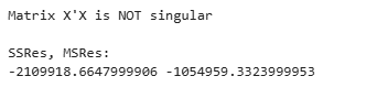
This is just because of the intermediate rounding the numbers. That has an adverse effect and subsequent steps cannot be implemented