
Gradient
Consider a scalar valued function $f(\text{X})$ defined on $n$ variables; that is, $f: \mathbb{R}^n \to \mathbb{R}$, where $\text{X}=(x_1,x_2,\cdots, x_n)^T$ $= \begin{pmatrix} x_1 \\ x_2 \\ \vdots \\ x_n \end{pmatrix}_{n \times 1}$
The gradient of $f(\text{X})$ defined as:
$$ \nabla f(\text{X}) = \begin{pmatrix} \frac{\partial f}{\partial x_1} \\ \frac{\partial f}{\partial x_2} \\ \vdots \\ \frac{\partial f}{\partial x_n} \end{pmatrix}_{n \times 1} $$
Where $\frac{\partial f}{\partial x_i}$ is the partial derivative of $f$ with respect to $x_i$ for $i = 1, 2, \dots, n$.
Example 1:
For a function $f(\text{X}) = x_1^2 + x_2^2 + \dots + x_n^2$, the gradient is:
$$ \nabla f(\text{X}) = \begin{pmatrix} 2x_1 \\ 2x_2 \\ \vdots \\ 2x_n \end{pmatrix} $$
Jacobian
The Jacobian matrix is a generalization of the gradient for vector-valued functions. For a vector function $g: \mathbb{R}^n \to \mathbb{R}^m$, where $\text{X} = \begin{pmatrix} x_1 \\ x_2 \\ \vdots \\ x_n \end{pmatrix}$ is an $n$-dimensional vector, and the output is a vector $\mathbf{y} = \begin{pmatrix} y_1 \\ y_2 \\ \vdots \\ y_m \end{pmatrix}$ in $\mathbb{R}^m$
That is,
$$y_1=f_1(x_1,x_2, \cdots, x_n)$$
$$y_2=f_2(x_1,x_2, \cdots, x_n)$$
$$\ddots \quad \ddots \quad \ddots \quad \ddots \quad \ddots$$
$$y_m=f_m(x_1,x_2, \cdots, x_n)$$
Then, the Jacobian matrix $J=[\frac{\partial y_i}{\partial x_j}]_{i=1,2,\cdots, m;\quad j=1,2,\cdots, n}$ is defined as:
$$ J = \begin{pmatrix} \frac{\partial y_1}{\partial x_1} & \frac{\partial y_1}{\partial x_2} & \dots & \frac{\partial y_1}{\partial x_n} \\ \frac{\partial y_2}{\partial x_1} & \frac{\partial y_2}{\partial x_2} & \dots & \frac{\partial y_2}{\partial x_n} \\ \vdots & \vdots & \ddots & \vdots \\ \frac{\partial y_m}{\partial x_1} & \frac{\partial y_m}{\partial x_2} & \dots & \frac{\partial y_m}{\partial x_n} \end{pmatrix}_{m \times n} $$
$$J_{ij}=\dfrac{\partial f_i(x_1, x_2,\cdots,x_n)}{\partial x_j} $$
Each entry $\frac{\partial y_i}{\partial x_j}$ is the partial derivative of the $i$-th output component $y_i$ with respect to the $j$-th input component $x_j$.
Example 2:
For a vector function $g(\text{X}) = \begin{pmatrix} x_1^2 + x_2 \\ x_1 x_2 \end{pmatrix}$, the Jacobian matrix is:
$$J(\text{X}) = \begin{pmatrix} 2x_1 & 1 \\ x_2 & x_1 \end{pmatrix} $$
Hessian
The Hessian matrix is a square matrix of second-order partial derivatives of a scalar-valued function $f: \mathbb{R}^n \to \mathbb{R}$ defined on a vector $\text{X}=(x_1,x_2,\cdots, x_n)^T$. Then, the Hessian matrix is defined as:
$$H[f] (or) H_f(\text{X}) = \begin{pmatrix} \frac{\partial^2 f}{\partial x_1^2} & \frac{\partial^2 f}{\partial x_1 \partial x_2} & \dots & \frac{\partial^2 f}{\partial x_1 \partial x_n} \\ \frac{\partial^2 f}{\partial x_2 \partial x_1} & \frac{\partial^2 f}{\partial x_2^2} & \dots & \frac{\partial^2 f}{\partial x_2 \partial x_n} \\ \vdots & \vdots & \ddots & \vdots \\ \frac{\partial^2 f}{\partial x_n \partial x_1} & \frac{\partial^2 f}{\partial x_n \partial x_2} & \dots & \frac{\partial^2 f}{\partial x_n^2} \end{pmatrix}_{n \times n}$$
Where each entry $\frac{\partial^2 f}{\partial x_i \partial x_j}$ is the second partial derivative of $f$ with respect to $x_i$ and $x_j$.
Example 3:
For a function $f(\text{X}) = x_1^2 + x_2^2$, the Hessian matrix is:
$$H_f(\text{X}) = \begin{pmatrix} 2 & 0 \\ 0 & 2 \end{pmatrix}$$
This Hessian matrix represents the second derivatives of $f$ with respect to each component of $\text{X}$.
Remark:
Hessian is the Jacobian of Gradient
$$H=J(\nabla f(x))$$
Summary
- The gradient is a vector $(n \times 1)$ of first-order partial derivatives of a scalar-valued function $f(x_1,x_2\cdots,x_n)$.
- The Hessian is a square matrix $(n \times n)$ of second-order partial derivatives of a scalar-valued function $f(x_1,x_2\cdots,x_n)$.
- The Jacobian is a $m \times n$ matrix of first-order partial derivatives for vector-valued function $\text{Y}=f(\text{X})$.
First Derivative Test:
The analytical first derivative test classifies extrema by checking how the sign of the derivative changes around a critical point.
The analytical first derivative test determines whether a point is a maximum or minimum by checking how the slope (gradient) changes sign from -ve to +ve for a minimum, and from +ve to -ve for maximum.
Purpose:
At a critical point, does the function change from decreasing to increasing or vice versa?
Steps:
- Compute $f'(x)$
- Find points where $f'(x) = 0$ or $f'(x)$ does not exist
- Check the sign of $f'(x)$
- $f'(x) > 0$ $f$ is increasing
- $f'(x) < 0$ $f$ is decreasing
- Check the sign changes around critical point, $c$
- Local Min:
- $x < c$, $f'(x) < 0$ $f$ is decreasing
- $x > c$, $f'(x) > 0$ $f$ is increasing
- Local max
- $x < c$, $f'(x) > 0$ $f$ is increasing
- $x > c$, $f'(x) < 0$ $f$ is decreasing
- Local Min:
Requirement: “No iteration”
- Compute $f'(x)$ symbolically.
- Solve $f'(x) = 0$ exactly
- Check sign changes
Possible Risks:
In real time,
- $f(x)$ depends on millions of parameters
- $f'(x) = 0$ is a large nonlinear system
- No closed form may exist
- Computationally too costly.
What’s in the sight:
To optimize we need only the direction of movement of a (loss or cost) function. This may be approximate even.
So Gradient descend or Step size descend Advantage
$$f(x – \epsilon ~ \text{sign}\, f'(x)) < f(x)$$
$\epsilon$: step size. $\quad x_{k+1} = x – \epsilon~ \text{sign}\, f'(x)$
or
$x_{k+1} = x_k – \eta f'(x_k)$ which uses direction + magnitude
Step size teaches to take care only which direction decreases the function, and we always move in the decreasing direction.
If $f'(x) > 0$ then right increasing and left decreasing; similarly if $f'(x) < 0$ then right decreasing and left increasing
So $f'(x) > 0$ move left of $x$
$f'(x) < 0$ move right of $x$
Second Derivative Test:
The analytical second derivative test determines whether a critical point is minimum or maximum by examining the curvature of the function
- Positive curvature ($2^{nd}$ deriv $> 0$) indicates a local minimum
- Negative curvature ($2^{nd}$ deriv $< 0$) indicates a local maximum.
Geometrically, the second derivative test classifies a critical point by checking whether the function bends upward or downward at that point.
(i.e) test uses curvature information to confirm whether a stationary point is locally maximizing or minimizing.
What it is?
$f”(x)$ is the curvature of $f(x)$, tells how the slope itself is changing
If $f'(x) = g(x)$ then $f”(x) = g'(x)$. That is, gradient of first derivative of $f$ (slope).
Slope or gradient tells directions of movement.
Meaning of curvature:
- $f”(x) > 0$ curve bends upwards $\cup$ like a bowl.
Concave up $\simeq$ Convex - $f”(x) < 0$ curve bends downwards $\cap$
Implication for optimization:
At a critical point
- If $f”(c) > 0$ curve bends upwards then it will be a point of Local Minima.
- If on the other hand $f”(c) < 0$ then it will be a point of Local maxima
- If $f”(c) = 0$ then it will be a point of Flat / Ambiguous.
First + second derivatives:
If $f”(c) < 0$, the curvature is negative (concave downward). In this case, the function $f(x)$ decreases more rapidly than the gradient (given by $f'(c)$) predicts, and we can “see” a local maximum.
If $f”(c) > 0$, the curvature is positive (concave upward). In this case, the function $f(x)$ decreases more slowly than expected and eventually begins to increase, so we can “see” a local minimum.
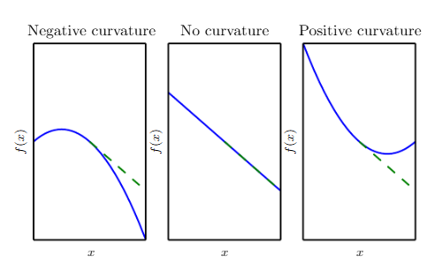
Figure 1: quadratic functions with various curvature
With no curvature, gradient “predicts” the decrease as Flat
$\therefore$ High Curvature $\to$ small steps
Low curvature $\to$ longer steps.
So, high curvature changes direction rapidly, so we must take small and cautious steps.
Low curvature changes direction slowly, so we can take longer and smoother steps.
Mathematically,
- $|f”(x)|$ large $\to$ smaller step
- $|f”(x)|$ small $\to$ longer step
Use in Newton’s method
$$x_{k+1} = x_k – \dfrac{f'(x_k)}{f”(x_k)}$$
Quick Fact:
Gradient says “Where should I go?”
Curvature says “How carefully should I go?”
“High Curvature in a loss function (surface) demands smaller optimization steps”
Use in “Scanning the space”:
In an $n$-D (parameter) space, it is not possible to “see” the whole landscape.
Like an interval in $\mathbb{R}^1$, area or box in $\mathbb{R}^2$ or cube in $\mathbb{R}^3$
But we probe locally using Gradient (Direction) and curvature (shape)
Each “step” updates our understanding of the space
Connection Between Hessian, and $2^{nd}$ order Derivatives
In high dimensional spaces, where the loss function can’t be “seen” (visualized), optimization proceeds by probing along chosen directions (locally $f’$)
- Restrict the function to a 1-D (chosen direction) curve, directional derivatives reduce the problem to “movement” along a line.
- Hessian ($H$) Characterizes how ‘$f$’ curves in every directions ($H$: matrix of $2^{nd}$ order partial derivation)
- Through the eigen decomposition of $H$, we have an orthogonal basis of principal directions.
- This allows all possible directional derivatives (curvatures) to be understood as combination of these Eigen vectors – fundamental axis.
From Goodfellow Book, p84, eqn 4.7
$$\dfrac{\partial^2 f}{\partial x_i \partial x_j} = \dfrac{\partial^2 f}{\partial x_j \partial x_i}$$
- $H$ is symmetric and real
- Decompose to set of real eigen values and an orthonormal basis of eigen vectors.
- The second derivative in a specific direction represented by a unit vector ‘$d$’ is $d^T H d$
If $d$ is eigen vector of $H$, then, the second derivative in that direction is given by corresponding Eigen vector.
$$d = \begin{bmatrix} d_1 \\ \vdots \\ d_n \end{bmatrix} \qquad d^T = [d_1\ d_2 \cdots d_n]$$
Then $$d^THd = [d_1\ d_2 \cdots d_n]_{1 \times n}\begin{bmatrix} \dfrac{\partial^2 f}{\partial x_1^2} & \dfrac{\partial^2 f}{\partial x_1 \partial x_2} & \cdots & \dfrac{\partial^2 f}{\partial x_1 \partial x_n} \\[2mm] \dfrac{\partial^2 f}{\partial x_2 \partial x_1} & \dfrac{\partial^2 f}{\partial x_2^2} & \cdots & \dfrac{\partial^2 f}{\partial x_2 \partial x_n} \\ \vdots & & & \vdots \\ \dfrac{\partial^2 f}{\partial x_n \partial x_1} & \dfrac{\partial^2 f}{\partial x_n \partial x_2} & \cdots & \dfrac{\partial^2 f}{\partial x_n^2} \end{bmatrix}_{n \times n}\begin{bmatrix} d_1 \\ d_2 \\ \vdots \\ d_n \end{bmatrix}_{n \times 1}$$
Let $n = 2$, $$X = \begin{bmatrix} x_1 \\ x_2 \end{bmatrix} \quad d = \begin{bmatrix} dx \\ dy \end{bmatrix} \text{ s.t. } \|d\| = 1$$
Let $t \in \mathbb{R}$ be a scalar
$$\therefore \quad td = \begin{bmatrix} t\,dx \\ t\,dy \end{bmatrix} \quad \text{and} \quad x + td = \begin{bmatrix} x_1 + t\,dx \\ x_2 + t\,dy \end{bmatrix}$$
Now $f: \mathbb{R}^2 \to \mathbb{R}$ implies
$$f(x + td) = f(x_1 + t\,dx,\ x_2 + t\,dy) \text{ which is a real number}$$
$$g(t) = f(x + td) = f(u(t), v(t))$$
$$\therefore \quad g'(t) = \dfrac{\partial f}{\partial u}\cdot\dfrac{du}{dt} + \dfrac{\partial f}{\partial v}\cdot\dfrac{dv}{dt} \text{ Implies}$$
$$g'(t) = \dfrac{\partial f(x+td)}{\partial x_1}\,dx + \dfrac{\partial f(x+td)}{\partial x_2}\cdot dy \tag{A}$$
$$\therefore \quad \nabla f(x + td) = \begin{bmatrix} \dfrac{\partial f}{\partial x_1} \\ \dfrac{\partial f}{\partial x_2} \end{bmatrix}$$
$$\Rightarrow \quad g'(t) = \nabla f(x+td)^T d$$
Using chain rule for each term in (A), for $g”(t)$
$$\dfrac{d}{dt}\left[\dfrac{\partial f}{\partial x_1}\right] = \dfrac{\partial}{\partial x_1}\left[\dfrac{\partial f}{\partial x_1}\,dx\right] + \dfrac{\partial}{\partial x_2}\left[\dfrac{\partial f}{\partial x_1}\cdot dy\right] \text{ similar to (A)}$$
$$\dfrac{d}{dt}\left[\dfrac{\partial f}{\partial x_2}\right] = \dfrac{\partial}{\partial x_1}\left[\dfrac{\partial f}{\partial x_2}\,dx\right] + \dfrac{\partial}{\partial x_2}\left[\dfrac{\partial f}{\partial x_2}\,dy\right]$$
$\therefore$ equ (A) become
$$g”(t) = dx^2\,\dfrac{\partial^2 f}{\partial x_1^2} + 2\,dx\,dy\,\dfrac{\partial^2 f}{\partial x_1 \partial x_2} + dy^2\,\dfrac{\partial^2 f}{\partial x_2^2}$$
$$= [dx\ \ dy]\,H\begin{bmatrix} dx \\ dy \end{bmatrix} = d^THd$$
$d^THd$ is a second order directional derivative that generalizes the 1-D second derivative along an arbitrary direction in $n$-D
Example 4: Gradient (2×2 Matrix)
The gradient of a scalar function $ f(x, y) $ is a vector that contains the partial derivatives of the function with respect to each variable.
Consider the function:
$$f(x, y) = x^2 + 3xy + y^2$$
The gradient $ \nabla f(x, y) $ is given by:
$$\nabla f(x, y) = \begin{bmatrix} \frac{\partial f}{\partial x} \\ \frac{\partial f}{\partial y} \end{bmatrix}$$
Now, we compute the partial derivatives:
- Partial derivative with respect to $ x $:
$$\frac{\partial f}{\partial x} = 2x + 3y$$ - Partial derivative with respect to $ y $:
$$\frac{\partial f}{\partial y} = 3x + 2y$$
Thus, the gradient is:
$$\nabla f(x, y) = \begin{bmatrix} 2x + 3y \\ 3x + 2y \end{bmatrix}$$
If we want to evaluate the gradient at the point $ (x, y) = (1, 2) $:
$$\nabla f(1, 2) = \begin{bmatrix} 2(1) + 3(2) \\ 3(1) + 2(2) \end{bmatrix} = \begin{bmatrix} 2 + 6 \\ 3 + 4 \end{bmatrix} = \begin{bmatrix} 8 \\ 7 \end{bmatrix} $$
Example 5: Jacobian (2×2 Matrix)
The Jacobian matrix is the matrix of all first-order partial derivatives of a vector-valued function. If you have a vector function $ \mathbf{F}(x, y) = \begin{bmatrix} f_1(x, y) \\ f_2(x, y) \end{bmatrix} $, the Jacobian matrix $ \mathbf{J}(x, y) $ is defined as:
$$ \mathbf{J}(x, y) = \begin{bmatrix} \frac{\partial f_1}{\partial x} & \frac{\partial f_1}{\partial y} \\ \frac{\partial f_2}{\partial x} & \frac{\partial f_2}{\partial y} \end{bmatrix} $$
Consider the vector function:
$$ \mathbf{F}(x, y) = \begin{bmatrix} f_1(x, y) \\ f_2(x, y) \end{bmatrix} = \begin{bmatrix} x^2 + 3xy \\ 2xy + y^2 \end{bmatrix} $$
Now, we compute the partial derivatives:
- For $ f_1(x, y) = x^2 + 3xy $:
- $$\frac{\partial f_1}{\partial x} = 2x + 3y$$
- $$\frac{\partial f_1}{\partial y} = 3x$$
- For $ f_2(x, y) = 2xy + y^2 $:
- $$\frac{\partial f_2}{\partial x} = 2y$$
- $$\frac{\partial f_2}{\partial y} = 2x + 2y$$
Thus, the Jacobian matrix is:
$$ \mathbf{J}(x, y) = \begin{bmatrix} 2x + 3y & 3x \\ 2y & 2x + 2y \end{bmatrix} $$
If we evaluate the Jacobian at $ (x, y) = (1, 2) $:
$$ \mathbf{J}(1, 2) = \begin{bmatrix} 2(1) + 3(2) & 3(1) \\ 2(2) & 2(1) + 2(2) \end{bmatrix} = \begin{bmatrix} 2 + 6 & 3 \\ 4 & 2 + 4 \end{bmatrix} = \begin{bmatrix} 8 & 3 \\ 4 & 6 \end{bmatrix} $$
Example 6: Hessian (2×2 Matrix)
The Hessian matrix is the square matrix of second-order mixed partial derivatives of a scalar function. If $ f(x, y) $ is a scalar function, the Hessian matrix $ H(x, y) $ is defined as:
$$ H(x, y) = \begin{bmatrix} \frac{\partial^2 f}{\partial x^2} & \frac{\partial^2 f}{\partial x \partial y} \\ \frac{\partial^2 f}{\partial y \partial x} & \frac{\partial^2 f}{\partial y^2} \end{bmatrix} $$
For the function:
$$ f(x, y) = x^2 + 3xy + y^2 $$
We compute the second-order partial derivatives:
- Second derivative with respect to $ x $:
$$ \frac{\partial^2 f}{\partial x^2} = 2 $$ - Mixed partial derivative $ \frac{\partial^2 f}{\partial x \partial y} $:
$$ \frac{\partial^2 f}{\partial x \partial y} = 3 $$ - Mixed partial derivative $ \frac{\partial^2 f}{\partial y \partial x} $:
$$ \frac{\partial^2 f}{\partial y \partial x} = 3 $$ - Second derivative with respect to $ y $:
$$ \frac{\partial^2 f}{\partial y^2} = 2 $$
Thus, the Hessian matrix is:
$$ H(x, y) = \begin{bmatrix} 2 & 3 \\ 3 & 2 \end{bmatrix} $$
Summary
We computed the gradient, Jacobian, and Hessian for the scalar and vector-valued functions.
- The gradient for $ f(x, y) = x^2 + 3xy + y^2 $ at $ (x, y) = (1, 2) $ is:
$$\nabla f(1, 2) = \begin{bmatrix} 8 \\ 7 \end{bmatrix} $$ - The Jacobian for $ \mathbf{F}(x, y) = \begin{bmatrix} x^2 + 3xy \\ 2xy + y^2 \end{bmatrix} $ at $ (x, y) = (1, 2) $ is:
$$ \mathbf{J}(1, 2) = \begin{bmatrix} 8 & 3 \\ 4 & 6 \end{bmatrix} $$ - The Hessian for $ f(x, y) = x^2 + 3xy + y^2 $ is:
$$ H(1, 2) = \begin{bmatrix} 2 & 3 \\ 3 & 2 \end{bmatrix} $$