
Functions of Single Variable
Parametric representations arise from the need to describe relationships where quantities evolve together through an underlying variable, often time, distance, exposure, or progression.
Instead of expressing one variable directly as a function of another, a parameter provides a natural way to capture the path, dynamics, and interaction between multiple processes. This approach is widely used when direct relationships are complex, hidden, or impossible to define explicitly.
A parametric representation describes two or more related quantities through a common underlying parameter t, rather than forcing a direct relationship between them: $x=x(t), y=y(t)$ where $t$ may represent time, progression, distance, exposure, or any driving process.
From physics and engineering to finance, biology, and genetics, parametric thinking helps represent evolving systems and derive meaningful rates such as (dy/dx) between related cumulative processes.
Example 1: Investement and Portfolio
Consider an investor’s portfolio over time: at any moment $t$, the portfolio’s value is $x(t)$, and $y(t)$ is the investor’s cumulative contribution into the portfolio.
$x$ nor $y$ is a function of the other directly — both are functions of $t$, and together, as $t$ moves forward, the pair $\big(x(t), y(t)\big)$ traces a path.
Here $\dfrac{dy}{dt}$ is the rate of investor contributions, and $\dfrac{dx}{dt}$ is the rate of change of portfolio value (contributions plus market movement).
Hence,
$$\frac{dy}{dx} = \frac{\text{contribution rate}}{\text{portfolio value growth rate}}$$
Finding $\frac{dy}{dx}$ – Differentiation of Inverse Functions
Consider a parametric representation: $x$ and $y$ are each given as $x = x(t), y = y(t)$.
Let us derive the the relationship between $x$ and $y$ themselves, if one is even needed, is only recovered indirectly, through their shared dependence on $t$. Following is a schematic representation of this relationships
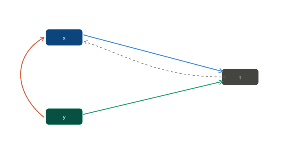
With reference to the above figure depicting this relationship between $x, y, t$, the red arrow indicates the relation of $y \to x$, and that arrow will be the path for $\dfrac{dy}{dx}$.
It breaks into two legs through $t: y \xrightarrow{\text{leg 1}} t \xrightarrow{\text{leg 2}} x$
So directly, $\frac{dy}{dx} = \underbrace{\frac{dy}{dt}}_{\text{leg 1}} \times \underbrace{\frac{dt}{dx}}_{\text{leg 2}}$
Inverse trick – Refer here
The diagram’s solid (blue) arrow gives us $x \to t$ directly, i.e. $\dfrac{dt}{dx}$ and the inverse is denoted by the dashed line. That is, $\dfrac{dx}{dt}$.
Now using the derivative of inverse functions, we can see that $\frac{dt}{dx} = \frac{1}{dx/dt}$
Substituting into the route:
$$\frac{dy}{dx} = \frac{dy}{dt}\times\frac{1}{dx/dt}$$
$$\boxed{\frac{dy}{dx} = \frac{dy/dt}{dx/dt}}$$
The rate of change of $y$ with respect to $x$ along this path, (Refer Example 1, how the portfolio’s value responds to contributions, even though neither was ever written as a direct function of the other) is found through the chain rule, treating $t$ as the connecting variable:
$$\frac{dy}{dx} = \frac{dy/dt}{dx/dt}$$
Example: Continuing the Investment Portfolio case, suppose contributions grow steadily, $y(t) = 5000t$, while the portfolio value grows as $x(t) = 2000t^2 + 1000$.
$$\frac{dy}{dt} = 5000, \qquad \frac{dx}{dt} = 4000t$$
$$\frac{dy}{dx} = \frac{5000}{4000t} = \frac{5}{4t}$$
At $t=1$, $\dfrac{dy}{dx} = \dfrac{5}{4} = 1.25$ — at this moment, contributions are increasing $1.25$ times as fast as portfolio value is, relative to each other, even though neither quantity was ever expressed directly in terms of the other; the comparison only exists through their common dependence on time.
Example: $\dfrac{dy}{dx}$ is Meaningful for a Parametric Pair
Suppose $\frac{dx}{dt} = 0.08x + 100, \qquad \frac{dy}{dt} = 100$
Then $\frac{dy}{dx} = \frac{100}{0.08x+100}$
The two extremes can be observed,
- When the portfolio is small, $x \approx 0$, so $\dfrac{dy}{dx} \approx \dfrac{100}{100} = 1$ — almost all of the increase in portfolio value comes from new contributions.
- As the portfolio grows large, $0.08x$ dominates the denominator, so $\dfrac{dy}{dx} \to 0$ — almost all of the increase comes from investment returns rather than new money being added.
This has a direct financial interpretation: the same formula smoothly captures the shift from “growth driven by saving” to “growth driven by compounding,” without needing a separate explanation for each regime.
Geometric Interpretation
If cumulative contributions $y$ are plotted against portfolio value $x$, then $\dfrac{dy}{dx}$ is the slope of that curve, and each value of the slope has a direct reading:
- $\dfrac{dy}{dx} = 1$: every dollar increase in portfolio value comes entirely from new contributions.
- $\dfrac{dy}{dx} = 0$: the portfolio is growing with no additional contributions at all — growth from returns alone.
- $0 < \dfrac{dy}{dx} < 1$: growth is a mixture of contributions and investment returns.
- $\dfrac{dy}{dx} > 1$: portfolio value is falling while contributions continue — possible during a market decline, where the denominator $dx/dt$ has become small or negative.
So mathematically, $\dfrac{dy}{dx}$ a contribution intensity — the fraction of the portfolio’s instantaneous change that is explained by new cash inflows rather than investment performance.
It is not a standard named metric in portfolio theory, but it is a meaningful derived quantity, built entirely from the parametric machinery already established.
Extending the Parametric Path
The examples above trace how $x$ and $y$, each a function of a single parameter $t$, yield $\dfrac{dy}{dx}$ through the two-legged chain $y \to t \to x$. A natural extension arises when $x$ and $y$ are themselves driven not by a single quantity but by two independent variables $u$ and $v$.
Consider the following use cases
Example 1:
A portfolio manager wants to understand how market conditions drive the overall growth rate of a fund. Two market forces act as the independent inputs. They do not directly determine the growth rate — instead they first shape two intermediate financial quantities, which in turn determine the single destination: the fund’s overall growth rate.
– $u$ : interest rate
– $v$ : inflation rate
– $x$ : bond yield (a function of interest rate and inflation)
– $y$ : equity return (a function of interest rate and inflation)
– $t$ : overall portfolio growth rate (determined through bond yield and equity return)
—
Example 2:
The same portfolio setting now tracks two destination quantities instead of one. The manager is not only interested in total return but also in portfolio risk. The same two market forces feed through the same two intermediate quantities, but now they jointly determine two outputs.
– $u$ : interest rate
– $v$ : inflation rate
– $x$ : bond yield (a function of interest rate and inflation)
– $y$ : equity return (a function of interest rate and inflation)
– $p$ : total portfolio return (destination 1)
– $q$ : portfolio risk or volatility (destination 2)
—
Example 3:
In a recommendation system, raw user behaviour signals are available. These signals do not directly predict user satisfaction — they first pass through two engineered features, which together determine a single prediction score.
– $u$ : number of clicks by the user
– $v$ : time spent on the platform
– $x$ : engagement score (derived from clicks and time)
– $y$ : bounce probability (derived from clicks and time)
– $t$ : predicted conversion probability (the single model output, reached through engagement score and bounce probability)
—
Example 4:
In a multi-task learning model, the same raw signals and the same intermediate feature representations now drive two separate prediction outputs simultaneously. This is common when a shared feature layer feeds into multiple output heads.
– $u$ : number of clicks by the user
– $v$ : time spent on the platform
– $x$ : engagement score (derived from clicks and time)
– $y$ : bounce probability (derived from clicks and time)
– $p$ : predicted conversion probability (destination 1)
– $q$ : predicted session depth (destination 2)
Generalizing these four cases:
Consider $x = x(u, v)$ and $y = y(u, v)$, where both $x$ and $y$ depend on the pair $(u, v)$.
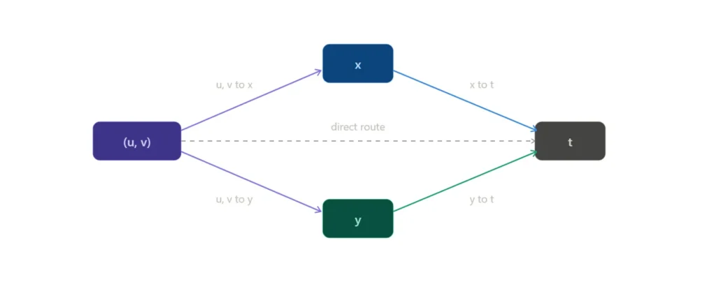
$(u, v)$ feeds into $x$ and $y$ separately, and $x$ and $y$ in turn connect to the single parameter $t$.
The diagram below captures this — the source node is the pair $(u, v)$, the intermediate nodes are $x$ and $y$, and the destination is still the single parameter $t$.
The two routes $u, v \to x \to t$ and $u, v \to y \to t$, along with the direct route, describe how the single parameter $t$ is reached through two different intermediate paths.
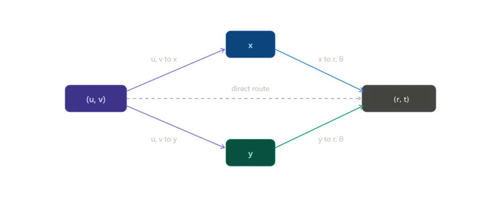
Cases three and four leads to a further generalisation. Instead of collapsing into a single parameter $t$ on the right, suppose the destination is itself a pair $(r, t)$.
Now $x$ and $y$ each carry information from $(u, v)$ on the left and route it toward $(r, t)$ on the right. The intermediate nodes $x$ and $y$ now relay between two independent inputs and two destination parameters, making the structure fully two-to-two.
The diagram below illustrates this: the routes $u, v \to x \to r, t$ and $u, v \to y \to r, t$ show how the pair $(r, t)$ is reached, with the direct route from $(u, v)$ to $(r, t$ still present as before.
Questions
- The overall portfolio growth rate $t$ responds to changes in bond yield $x$ and equity return $y$, both of which are themselves shaped by interest rate $u$ and inflation $v$. How does the portfolio growth rate change as inflation rises, accounting for the fact that inflation simultaneously affects both channels?
- At a moment when interest rate $u$ is held fixed, how does a unit change in inflation $v$ propagate through equity return $y$ alone to affect portfolio growth $t$?
- Bond yield $x$ and equity return $y$ each respond to $u$ and $v$ independently. Is the combined effect of both inputs on portfolio growth $t$ simply the sum of their individual effects? What mathematical object would tell you whether or not that is the case?
- Suppose portfolio growth $t$ is accelerating with respect to interest rate $u$. What does that require of the intermediate quantities $x$ and $y$, and what kind of information about them is needed to answer this?
- Total return $p$ and portfolio risk $q$ are both shaped by bond yield $x$ and equity return $y$. If inflation $v$ increases slightly, how do $p$ and $q$ move relative to each other — do they move together, in opposite directions, or independently? What would you need to compute to answer this?
- A fund manager wants to know whether increasing interest rate $u$ improves return $p$ faster than it worsens risk $q$. What quantities need to be compared, and what is the nature of those quantities?
- How does the sensitivity of total return $p$ to inflation $v$ change as interest rate $u$ itself varies? What kind of rate captures this?
- If both $u$ and $v$ change simultaneously by small amounts, how would you express the resulting joint change in the pair $(p, q)$ together?
- Predicted conversion probability $t$ depends on engagement score $x$ and bounce probability $y$, both derived from clicks $u$ and time on page $v$. If time on page increases marginally while clicks remain fixed, how does conversion probability respond, and through which intermediate does that response travel?
- A model audit finds that conversion probability $t$ is highly sensitive to clicks $u$ at low engagement, but insensitive at high engagement. What mathematical property of the relationship between $t$ and $u$ — through $x$ and $y$ — describes this changing sensitivity?
- Engagement score $x$ and bounce probability $y$ are both functions of clicks $u$ and time $v$. Does the order in which you account for $u$ and $v$ matter when studying how they jointly shape $t$? What condition on the intermediates determines this?
- Predicted conversion $p$ and predicted session depth $q$ are both outputs of the same shared feature layer built from clicks $u$ and time $v$. If clicks increase by a small amount, how do the two predictions shift relative to each other? Are their sensitivities to $u$ necessarily related, or can they move independently?
- A model retraining changes how engagement score $x$ responds to time on page $v$. Which of the two outputs $p$ and $q$ is more affected, and what would you compute to find out?
- Suppose session depth $q$ appears stable with respect to clicks $u$ at a particular operating point, but the analyst suspects this stability breaks down as time on page $v$ grows large. What mathematical object captures whether and how the sensitivity of $q$ to $u$ itself changes with $v$?
- The two outputs $p$ and $q$ share the same inputs $u$ and $v$ through the same intermediates $x$ and $y$. Under what conditions would a change in $v$ affect $p$ and $q$ by exactly the same amount, and what does that imply about the structure of the model?