
Introduction
This notes confines to MLE in obtaining Point Estimators for parameters
Suggested Reading: [CABE] Casella, G., & Berger, R. L. (2002). Statistical inference (Vol. 2). Pacific Grove, CA: Duxbury; specifically, Chapters 6 and 7
For calculus Review: [TOFI] Thomas, G. B., & Finney, R. L. Calculus and analytic geometry. Addison Wesley Publishing Company.
Keywords:
- Estimator
- Estimate
- Likelihood function
- Method of Moments (MOM)
- Maximum Likelihood Estimates (MLE)
- Bias, Variance and Mean Squared Error (MSE) of an estimator
Objectives
- Method of finding estimators
- Criteria to find a “best” estimator
- Assessing tools – goodness of estimator
Symbols followed
- $\theta:$ Parameter
- $f(x_i|\theta):$ Probability density/mass function
- $L(\theta|X):$ Likelihood function
- $l(\theta|X)= \ln L(\theta|X):$ Log Likelihood function
An estimator of $\tau(\boldsymbol\theta)$, a function of parameter is any function $W(X_1,X_2,\cdots,X_n)$ of a sample; that is any statistic is a point estimator
Here, $\boldsymbol{\theta}=(\theta_1, \theta_2,\cdots,\theta_k)$
Maximum Likelihood Estimators
The process of MLE is to maximize the likelihood function $L(\theta~|~X) = f(X~|~\theta)$, the joint pdf or pmf of the sample X
that is to find a parameter value $\hat\theta(X)$ at which $L(\theta~|~X)$ attains its maximum as a function of $\theta$
First, we consider the analytical method (calculus approach) using second derivative test to find maximum of a function.
However, second derivatives are not explicitly derived in this note and left as an exercise.
Examples of MLE
Example 1: Bernoulli Distribution
Let $X_1,X_2,\cdots,X_n \sim \text{Bernoulli} (\theta)~~~~~~~ x = 0,~1;~~~~ 0 < \theta<1$
$f(x_i|\theta) = \theta^{x_i} (1-\theta)^{1-x_i} ~~~~~ i = 0,~1$
$\Rightarrow L(\theta|X) = \prod_{i=1}^n f(x_i|\theta)$
$L(\theta|X) =\prod_{i=1}^n \theta^{x_i} (1-\theta)^{1-x_i}$
$L(\theta|X) = \theta^{\sum x_i} (1-\theta)^{n-{\sum x_i}}$
$l(\theta|X) = \sum x_i ~\ln\theta +(n-\sum x_i) ~~\ln(1-\theta)$
$\frac{dl}{d\theta} = \sum x_i \frac{1}{\theta} + \frac{(n-\sum x_i)}{1-\theta} (-1)$
$\frac{dl}{d\theta} = 0$
$\Rightarrow \frac{1}{\theta}\sum x_i – \frac{n-\sum x_i}{1-\theta} = 0$
$\Rightarrow (1-\theta) \sum x_i – (n-\sum x_i) \theta = 0$
$\Rightarrow \sum x_i – n\theta = 0$
$\hat\theta_{ML} = \frac{\sum x_i}{n} = \overline {X}$
Example 2 Poisson Distribution
$X_1,\cdots,X_n \sim \text{Poisson}(\theta)$
$f(x_i~|~\theta) = e^{-\theta}~ \frac{\theta~^{x_i}}{x_i~!}$
$L(\theta|X) = \prod e^{-\theta}~ \frac{\theta~^{x_i}}{x_i!}$
$=e^{-n\theta}~ \frac{\theta~^{\sum x_i}}{\prod x_i!}$
$l(\theta|X) = -n~\theta + \sum x_i \ln \theta + k$
$\frac{\partial~l}{\partial~\theta} = 0$
$\Rightarrow -n + \sum x_i~ \frac{1}{\theta} = 0$
$\Rightarrow n =\frac{\sum x_i}{\theta}$
$\Rightarrow \hat\theta_{ML} = \overline {X}$
Example 3: Geometric Distribution
Let $X_1,X_2,\cdots,X_n \sim \text{Geometric}~(\theta)$
$\Rightarrow f(x_i,\theta) = \theta (1-\theta)^{x_i -1 } ~~~x_i = 1,2,3,…$
$L(\theta|X) = \prod_{i=1}^{n} \theta (1-\theta)^{x_i -1}$
$L(\theta|X) = \theta^n (1-\theta)^{\sum x_i-n}$
$l(\theta|X) = n \ln \theta + (\sum x_i – n ) \ln(1-\theta)$
$\frac{dl}{d\theta} = n \frac{1}{\theta} + \frac{\sum x_i -n}{1-\theta} (-1)$
$\frac{dl}{d\theta} = 0$
$\Rightarrow \frac{n}{\theta} -\frac{\sum X_i – n}{1-\theta} = 0$
$\Rightarrow n(1-\theta) – (\sum X_i – n) \theta = 0$
$\Rightarrow n – (\sum x_i) \theta = 0$
$\hat\theta_{ML} = \frac{n}{\sum x_i} = \frac{1}{\overline{X}}$
Example 4: Gamma Distribution
Let $X_1,\cdots,X_n \sim \text{Gamma}~(\alpha,\beta)$ $X>0$ Assume $\alpha$ is known
$L(\theta|X) = \prod f(x_i~|~\theta)$ $\theta = \beta >0$ which is a scale parameter
$L(\theta|X) = \prod_{i=1}^n \frac{1}{\Gamma\alpha~\beta^\alpha}~ x_i~^{\alpha – 1}~ \exp\Big[-\frac{x_i}{\beta}\Big]$
$= (\frac{1}{\Gamma \alpha})^n \beta^{-\alpha~n}~ \prod x_i~^{\alpha-1} \exp\Big[-\frac{x_i}{\beta}\Big]$
$l(\theta|x) = k -~ \alpha~n~\ln\beta + (\alpha -1 )~\sum \log X_i – \frac{\sum \alpha_i}{\beta}$ where $k$ is a constant free from the parameter $\beta$
$\frac{\partial~l}{\partial~\beta} = 0$
$\Rightarrow -~\alpha~n~ \frac{1}{\beta} + \frac{\sum X_i}{\beta^2} = 0$
$\frac{\sum X_i}{\beta} = -\alpha~n$
$\Rightarrow \hat\beta_{ML} = \frac{\sum X_i}{\alpha~n}$
$\hat\beta_{ML}= \frac{\overline {X}}{\alpha}$
If $\alpha >0$ is also unknown.
$l(\theta|x) = -n~\ln \Gamma\alpha ~-~\alpha~n~\ln \beta + (\alpha -1) \sum \ln X_i – \frac{\sum X_i}{\beta}$ and $\theta= \alpha ~ \& ~ \beta$
$\frac{\partial~ l}{\partial~ \alpha} = 0$
$\Rightarrow -\frac{n~(\Gamma \alpha)’}{\Gamma \alpha} – n~\ln \overline {X} + \alpha~n~\frac{1}{\alpha} + n~\ln \alpha + \sum \ln X_i – n = 0$
$\Rightarrow n~\log \alpha – \frac{n~(\Gamma\alpha)’}{\Gamma \alpha} = n~\ln \overline {X} – \sum \ln x_i$
$\Rightarrow \ln \alpha – \frac{(\Gamma\alpha)’}{\Gamma \alpha} = \ln \overline {X} – \frac{\sum \ln x_i}{n}$
solving this equation in $\alpha$ provides ML estimator for $\alpha$
Example 5: Exponential Distribution
$X_1,\cdots,X_n \sim \text{Exponential}(\theta)$
$f(x~|~\theta) = \theta~e^{-\theta x}~~~~~~~x>0;~~~~\theta>0$
$L(\theta|X) = \prod_{i=1}^{n} f(x_i~|~\theta)$
$L(\theta|X) = \prod \theta~e^{-\theta x_i}$
$L(\theta|X) = \theta^n e^{-\theta\sum x_i}$
$l(\theta|X) = n~\ln \theta – \theta \sum x_i$
$\frac{dl}{d\theta} = 0$
$\Rightarrow \frac{n}{\theta} – \sum x_i = 0$
$\Rightarrow \frac{n}{\theta} = \sum x_i$
$\Rightarrow \hat\theta_{ML} = \frac{n}{\sum x_i} = \frac{1}{\overline {X}}$
Example 6: Negative Binomial Distribution
Let $X_1,\cdots,X_n \Rightarrow NBD(r;\theta)$
If x is the number of trials required to get $r$ successes in a sequence of Bernoulli experiment
$f(x_i~|~\theta)= {x_{i}- 1~ \choose r-1}~ \theta^r~ (1-\theta)^{x_i – r} ~~~ x_i = r,r+1,\cdots$
$L(\theta|X) = \prod_{i=1}^n {x_i -1 \choose x_i -r} \theta^r (1-\theta)^{x_i – r}$
$= \theta^{nr} (1-\theta)^{\sum x_i – nr} \prod {x_i -1 \choose x_i – r}$
$l(\theta|X) = n~r\ln\theta + (\sum x_i – n~r)~\ln (1-\theta) + k$
$\frac{\partial~l}{\partial~ \theta} = 0 \Rightarrow$
$\frac{n~r}{\theta} + \frac{\sum x_i – n~r}{1-\theta}(-1) = 0$
$n~r(1-\theta) – (\sum x_i – nr) \theta = 0$
$\Rightarrow n r – \theta\sum x_i = 0$
$\hat\theta_{ML} = \frac{nr}{\sum x_i}$
$\hat\theta_{ML} = \frac{r}{\bar X}$
If $x_i$ referes the number of failures preceeding rth successes, then
$f(x_i~|~\theta) = {x_i~+~r-1~~\choose r-1}~ \theta^r~(1-\theta)^{x_i} ~~~~x = 0,1,2,\cdots$
$L(\theta|X) = \prod {x_i+r-1~ \choose r-1} ~\theta^r ~(1-\theta^{x_i}) ~~~~ x_i = 0,1,2,\cdots$
$= \theta^{nr}~ (1-\theta)^{\sum x_i}~ \prod {x_i+r-1~ \choose x_i}$
$l(\theta|X) = n~r~\ln \theta + \sum x_i~ \ln(1-\theta) + k$
$\frac{\partial~l}{\partial~\theta} = 0 \Rightarrow$
$\frac{nr}{\theta} + \frac{\sum x_i}{1-\theta}(-1) = 0$
$\Rightarrow n~r~(1-\theta) – (\sum x_i)~\theta = 0$
$\Rightarrow n~r-n~r~\theta – (\sum x_i) ~\theta = 0$
$\Rightarrow n~r – \theta(n~r+\sum x_i) = 0$
$\Rightarrow \theta_{MLE} = \frac{n~r}{n~r+\sum x_i}$
$= \frac{n~r}{\sum(x_i + r)}$
$=\frac{n~r}{\sum y_i}$
$\hat\theta_{ML} = \frac{r}{\bar y}$
Even if $x_i$ is defined in different manner, MLE of the proportion parameter is same
Also to note that when r = 1, we get MLE for the parameter in Geometric distribution.
Example 7: Beta Distribution
Let $X_1,X_2,\cdots,X_n) \sim \text{Beta}(1,\theta)$
$\Rightarrow f(x_i ~|~\theta) = \theta (1-x_i)^{\theta-1}~~~~~~~~~0 < x < 1;~ \theta>0$
$L(\theta|X) = \prod f(x_i ~|~\theta)$
$= \prod \theta (1-x_i)^{\theta-1}$
$=\theta^n \prod (1-x_i)^{\theta-1}$
$l(\theta|X) = n~\ln\theta + (\theta-1) \sum \ln(1-x_i)$
$\frac{\partial~l}{\partial~\theta} = 0$
$\Rightarrow \frac{n}{\theta} + \sum \ln (1-x_i) = 0$
$\Rightarrow \hat\theta_{ML} = \frac{n}{-\sum \ln (1-x_i)}$
Following situations help to understand the limitations of analytical method (calculus approach). Alternative approach is needed to maximize the likelihood functions
Example a.
Let $X_1,X_2,\cdots,X_n \sim U(\theta – 1/2,~\theta + 1/2)$
$f(x_i,\theta) = 1 ~~~~~~~\theta – 1/2 < x_i < \theta + 1/2$
$L(\theta|X) = \prod_{i=1}^n 1 ~~~~$ whenever $~~\theta – 1/2 < x_i < \theta + 1/2$
$i.e.~ Y_1 = Min X_i > \theta – 1/2$
$Y_n = Max X_i < \theta + 1/2$
or $Y_n – 1/2 < \theta < Y_1 + 1/2 ~~~~~~~~~~~~~~~~~~~~~~(1)$
Any $\theta$ satisfies $(1)$ could be an MLE
$\hat\theta_{ML} = \frac{Y_1+1/2+Y_n-1/2}{2}$
$= \frac{Y_n + Y_1}{2}$
This is average of maximum and minimum of X
This idea can be used to the following situations also
$X_1,X_2,\cdots,X_n \sim u(0,\theta)$ to obtain $\hat\theta_{ML} = Max X_n$
Example b.
Let $X_1,\cdots,X_n \sim u(\mu – \sqrt 3 \sigma , \mu + \sqrt 3 \sigma)$
$f(x_i,\theta) = \frac{1}{2\sqrt 3 ~\sigma} ~~~~$if $~\mu – \sqrt 3 \sigma < x_i < \mu + \sqrt 3 \sigma$
$\Rightarrow L(\theta|X) = \prod_{i=1}^n \frac{1}{2\sqrt3 \sigma}$
$L(\theta|X) = (\frac{1}{2\sqrt3 \sigma})^n ~~~~ x_i \in [ \mu – \sqrt3 \sigma ,\mu + \sqrt3 \sigma)$
Hence, minimum of X, $Y_1 > \mu – \sqrt3 \sigma$ and maximum of X $Y_n < \mu + \sqrt3 \sigma$
$\hat\mu_{ML} = \frac{Y_1+Y_n}{2}$
$\sqrt3 \sigma = Y_n – \mu$
$\sigma = Y_n – (\frac{Y_1 + Y_n}{2})$
$\sigma = \frac{Y_n – Y_1}{2 \sqrt3}$
Optimization for function of several variables
From Matrix Theory
Let $A = (a_{ij})_{n\times n}$. A $k \times k$ submatrix of A formed by deleting $n-k$ rows of $A$, and the same $n-k$ columns of $A$, is called $\textbf{principal sub matrix of A}$.
The determinant of a principal submatrix of A is called a $\textbf{principal minor}~\Delta_k$ of $A$.
The $\textbf{leading principal minor of A}$ of order $k$ is the minor of order $k$ obtained by deleting the last $n-k$ rows and columns. We denote leading principal minor of $A$ as $L\Delta_k$
For example, if $A = (a_{ij})_{2\times 2}$ then $L\Delta_1=a_{11}$ and $L\Delta_2= det(A)=a_{11}a_{22}-a_{21}a_{12}$
Let $A$ be a symmetric $n \times n$ matrix. Then we have:
1. $A$ is positive definite $\iff$ $L\Delta_k>0$ for all leading principal minors
2. $A$ is negative definite $\iff$ $(-1)^kL\Delta_k >0$ forall leading principal minors
Matrix Example 1:
Consider $$ A =\left(\begin{array}{cccc} 2 & -1 & 0 \\ -1 & 2 & -1 \\ 0 & -1 & 2 \end{array}\right) $$
$L\Delta_1=A_{11}=2$
$L\Delta_2= det\left(\begin{array}{cccc} 2 & -1 \\ -1 & 2\end{array}\right) = 3 $
$L\Delta_3=detA=4$
All $L\Delta_k$ are positive. $A$ is positive definite
Matrix Example 2:
Consider $$ A =\left(\begin{array}{cccc} 2 & -1 \\ -1 & -2 \end{array}\right) $$
$L\Delta_1=A_{11}=2>0$
$L\Delta_2=detA = -5<0$
$A$ is negative definite
Hessian Matrix
Let $f(\textbf{X})$ be a real valued function in $\mathbb{R^n}$ that is $f:\mathbb{R^n}\rightarrow\mathbb{R}$ $\textbf{X}=(x_1,x_2,\cdots,x_n)$
Gradient of $f$ is $\nabla f=\Big(\frac{\partial~f} {\partial~x_1},\frac{\partial~f} {\partial~x_2},\cdots,\frac{\partial~f} {\partial~x_n}\Big)$
Hessian matrix is $$H =\left(\begin{array}{cccc} f_{11} & f_{12} & \cdots & f_{1n} \\ f_{21} & f_{22} & \cdots & f_{2n} \\ \vdots & \vdots & \ddots & \vdots \\ f_{n1} & f_{n2} & \cdots & f_{nn} \end{array}\right) $$ where $f_{ij}=\frac{\partial^2~f} {\partial~x_i~\partial~x_j}~~\forall ~i, ~ j=1,2,\cdots,n$ and it is easy to observe that $f_{ij}=f_{ji}$ and $H$ is symmetric
Hessian Matrix and convexity
1. $H$ is Positive definite $\Rightarrow$ $f$ is convex
2. $H$ is Negative definite $\Rightarrow$ $f$ is concave
It is also to note that if $f$ is concave all stationary points $\{x_0/\nabla f(x_0)=0\}$ ($x_0$ is not on the boundary of the open set S) are global maximum points. Read for more details $\textbf{TOFI}$
Example: Bernoulli Likelihood with 5 trials and 3 observed successes
$l(\theta~|~X) = 3\ln\theta + 2 \ln (1-\theta)$ so that $\nabla f = \frac{3-5\theta}{\theta(1-\theta)}$ and $H=-\Big[\frac{3}{\theta~^2}+\frac{2}{(1-\theta)~^2}\Big]$
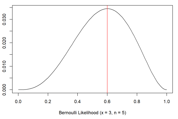
It is easy to observe that at $\theta = 0.6, \nabla f = 0$; if $\theta < 0.6, \nabla f > 0$ and if $\theta > 0.6, \nabla f < 0$
Also it can be observed that H is always negative.
This example illustrates the behaviour of $\nabla f$ and Hessian matrix near a local maximum as well as the notion of concavity.
Example:
$f(x_1,x_2) = x^2_1-x^2_2-3x_1x_2$ can easily be verified as a concave function by observing the Hessian matrix as negative definite $L\Delta_1=H_{11}>0$ and $L\Delta_2=\text{det}H <0$
$\textbf{NOTE: Maximization For Two Parameters}$ $\theta_1,~\theta_2$
1. Solve $\frac{\partial ~l}{\partial~\theta_1} = 0$ and $\frac{\partial~l}{\partial~\theta_2}=0$ for $\theta_1,~\theta_2$
2. Compute Hessian matrix.
3. Check whether $H$ is negative definite.
Example:Normal Distribution
Let $X_1,X_2,…,X_n \sim N(\mu,\eta) ~~~\eta=\sigma^2$
$L(\theta|X) = \prod f(x_i|\theta)$ where $\theta = \mu~\&~\eta$
$L(\theta|X) = \prod \Big[\frac{1}{\sqrt{2\pi\eta}}\Big] e^{-\frac{1}{2\eta}(X_i – \mu)^2}$
$L(\theta|X) = \Big[\frac{1}{\sqrt{2\pi\eta}}\Big]^n e^{-\frac{1}{2\eta}\sum(X_i – \mu)^2}$
$l(\theta|X) = k – \frac{n}{2} \ln \eta – \frac{1}{2\eta} \sum(X_i – \mu)^2$ where $k$ is constant free from parameters $\mu,\eta$
$\frac{\partial~l}{\partial~\mu} = 0$
$\Rightarrow -~\frac{1}{2\eta} 2\sum(X_i – \mu)^2 (-1) = 0$
$\Rightarrow \sum X_i -n\mu = 0$
$\Rightarrow \hat\mu = \overline {X}$
$\frac{\partial~l}{\partial~\eta} = 0$
$\Rightarrow -\frac{n}{2\eta} + \frac{1}{2\eta^2}\sum(X_i – \mu)^2 = 0$
$\Rightarrow \frac{1}{2\eta}\Big[-n + \frac{1}{\eta}\sum(X_i – \mu)^2\Big] = 0$
$\Rightarrow \frac{1}{\eta} \sum(X_i – \mu)^2 = n$
$\Rightarrow \eta = \frac{\sum(X_i – \mu)^2}{n}$
With $\hat\mu_{ML} = \overline {X}$ we have
$\hat \eta_{ML} = \widehat {\sigma^2_{ML}} =\frac{\sum(X_i – \overline {X})^2}{n}$