
Introduction
Random variable and theoretical distributions play very important role in modeling uncertainty. It offers a syntactic approach for the language of uncertainty. Many standard texts such as Casella and Berger on Mathematical Statistics and / or Statistical Inference deal with Distributions extensively. Fundamentals of dealing with uncertainty through a mathematical description or distribution and probability functions and relevant computations are discussed in this presentation.
Univariate Random Variables
Definition:
Given a random experiment with sample space $\mathbb{S}$. A function $X$, which assigns to each element $s$ in $\mathbb{S}$ one and only one real number $X(s)=x$, is called a random variable. The range or space of $X$ is the set of real numbers $\mathscr{A}_X$ such that $\mathscr{A}_X=\{ x \in \mathbb{R}/ X(s)=x, s \in \mathbb{S}\}$
If the set $\mathbb{S}$ has elements which are themselves real numbers, then we could write $X(c)=c$, so that $\mathscr{A}_X=\mathbb{S}$. On the other hand, if $\mathbb{S}$ has non-numerical elements then a random variable assigns a numerical value (of course, unique) to each of the elements of $\mathbb{S}$
Example 1
Let a coin be tossed thrice
$$\therefore \mathbb{S} = \{HHH, HHT, HTH, THH, HTT, THT, TTH, TTT\}$$
For simplicity we assume that $\mathbb{S}_i \ (i = 1 \text{ to } 8)$ denotes the $i^{th}$ outcomes i.e., $i^{th}$ elements in $\mathbb{S}$.
If our interest is in the number of heads in the $i^{th}$ outcome $(i = 1 \text{ to } 8)$.
i.e.,
$$X(\mathbb{S}_i) = \text{Number of heads in the } i^{th} \text{ outcome}$$
$$\therefore \quad X(\mathbb{S}_1) = 3 \quad X(\mathbb{S}_2) = X(\mathbb{S}_3) = X(\mathbb{S}_4) = 2$$
$$X(\mathbb{S}_5) = X(\mathbb{S}_6) = X(\mathbb{S}_7) = 1 \quad X(\mathbb{S}_8) = 0$$
Hence
$$\mathscr{A}_X = \{0, 1, 2, 3\}.$$
Example 2
Let us choose a real number randomly in an interval say $(0, 1)$. In this case $\mathbb{S}$ itself has real numbers as its elements.
$$\therefore \quad \text{we define} \quad X: \mathbb{S} \to \mathbb{R} \quad \text{s.t}$$
$$X(s) = s \quad \text{so that} \quad \mathscr{A}_X = (0, 1) \text{ or } \mathbb{S}.$$
Example 3
If a person randomly answers a ‘True or False’ question set then the sample space $\mathbb{S} = \{$’True’, ‘False’$\}$. In this case, define $X: \mathbb{S} \to \mathbb{R}$ as $X(\text{True}) = 1$ and $X(\text{False}) = 0$ so that $\mathscr{A}_X = \{0, 1\}$.
Example 4
In Example 3, if we are interested to count the number of times the person answered ‘True’ thus $\mathbb{S} = \{0, 1, 2, 3 \cdots\}$ (assuming that number of Questions is unknown). So that $\mathbb{S}$ has real numbers.
$$\therefore \quad \mathscr{A}_X = \mathbb{S}$$
Discussion
1. Examples 1 and 3 show how non-numerical elements are assigned with real numbers and Examples 2 and 4 are for numerical elements in sample space.
2. Examples 1 and 3 have finite space $A$ and Example 4 has a countably infinite space where as Example 2 has uncountably infinite space $A$. This idea formulates the two different types of random variables, as
Discrete random variables
Let $X$ be a random variable with one-dimensional space $\mathscr{A}_X$. If $\mathscr{A}_X$ has only a finite number of different values $x_1, x_2 \cdots x_k$ or at most countably infinite sequence of different values $x_1, x_2 \cdots$ then $X$ is said to be discrete random variables.
Continuous random variables
Let $X$ be a random variable with one-dimensional space $\mathscr{A}_X$. If $\mathscr{A}_X$ is a uncountably infinite set (as every value in an interval) then $X$ is said to be continuous random variable.
In general, countable quantities can be regarded as discrete random variables whereas measurable quantities (such as height, weight, voltage) can be considered as continuous random variables, of course, the variable in the problem possesses random nature.
Also, one can classify the nature of a random variable based only on the range $\mathscr{A}_X$ of $X$.
Probability Functions
For each random variable $X$ we have a set of real numbers $\mathscr{A}_X$. $X$ assumes its value in $\mathscr{A}_X$ we could calculate the probability that $X$ takes its value in $\mathscr{A}_X$. The collection of these probabilities is the distribution of $X$. Also, these distributions can be described by what we will call as probability Density Function (pdf).
For any random variable $X$ and its space $\mathscr{A}_X$ we call a new function $f_X(x)$ for all $x \in \mathscr{A}_X$ which has to satisfy the two conditions viz. (a) non-negativity, (b) Totality of $f_X(x) = 1$. Now, let use define precisely for the two types of random variables.
1. Discrete random variables
Let $X$ be a discrete random variable with space $\mathscr{A}_X$. Then $f_X(x)$ is defined on $\mathscr{A}_X$ such that
(a) $f_X(x) \geq 0$,
(b) $\displaystyle\sum_{x \in \mathscr{A}_X} f_X(x) = 1$.
2. Continuous random variables
Let $X$ be a continuous random variable with space $\mathscr{A}_X$. Then $f_X(x)$ is defined on $\mathscr{A}_X$ such that
(a) $f_X(x) \geq 0$,
(b) $\displaystyle\int_{\mathscr{A}_X} f_X(x) \, dx = 1$.
the probability function $f_X(x)$ of a discrete random variable is called as probability mass function (pmf) and that of a continuous random variable we call it as a probability density function (pdf).
It is seen that whether the random variable $X$ is of the discrete type or of the continuous type, the probability $p(X \in A)$ where $A \subseteq \mathscr{A}_X$ is completely determined by a function $f_X(x)$. On either case, we may work exclusively with the probability function $f_X(x)$.
Normalizing Constant
The PDF/PMF is fundamentally a mathematical function but to satisfy the two conditions – (i) Non- nagativity and (ii) total probability=1. Hence, the mathematical form of a function needs a way to satisfy these conditions.
for example, if continuos random variable has a function $f_X(x)$ with domain $\mathscr{A}$. Let $f_X(x) \geq 0$ but $\displaystyle\int_{\mathscr{A}_X} f_X(x) \, dx \neq 1$. In that case, we can make $g_X(x)=k f_X(x)$ where $k=\frac{1}{\displaystyle\int_{\mathscr{A}_X} f_X(x) \, dx}$ and $g(x)$ in $\mathscr{A}$ will become a valid PDF. Such constants are called Normalizing Constant. If it is a discrete random variable replace the integral with sum.
Example 5
If the pmf or pdf of a random variable $X$ is as follows:
$$ \text{(a)} \quad f_X(x) = \begin{cases} Cx^2 & 1 \leq x \leq 2 \\ 0 & \text{elsewhere} \end{cases} $$
$$ \text{(b)} \quad f_X(x) = \begin{cases} Ce^{-2x} & x > 0 \\ 0 & \text{elsewhere} \end{cases} $$
$$ \text{(c)} \quad f_X(x) = \begin{cases} Cx & x = 1, 2, 3, 4, 5 \\ 0 & \text{elsewhere} \end{cases} $$
$$ \text{(d)} \quad f_X(x) = \begin{cases} C & x = 1, 2, 3, \cdots, 10 \\ 0 & \text{elsewhere} \end{cases} $$
$\textbf{Solution}$
(a) $X$ is a continuous random variable since $\mathscr{A} = \{1, 2\}$.
$$\therefore \quad \int_\mathscr{A} f_X(x) \, dx = 1 \implies \int_1^2 Cx^2 \, dx = 1 $$
$$\implies C\left(\frac{x^3}{3}\right)_1^2 = 1 $$
$$ \implies C\left(\frac{8-1}{3}\right) = 1 $$
$$ \implies C = \frac{3}{7} $$
(b) In this case $\mathscr{A} = (0, \infty)$, so that $X$ is a continuous random variable, so that
$$ \int_\mathscr{A} f_X(x) \, dx = 1 \implies \int_0^{\infty} Ce^{-2x} \, dx = 1 $$
$$ \implies C\left(\frac{e^{-2x}}{-2}\right)_0^{\infty} = 1 $$
$$ \implies C\left(\frac{1-0}{2}\right) = 1 $$
$$ \implies C = 2 $$
(c) Here $\mathscr{A} = \{1, 2, 3, 4, 5\}$, hence $X$ is a discrete random variable, so that
$$ \sum_{x \in \mathscr{A}} f_X(x) = 1 \implies C(1) + C(2) + C(3) + C(4) + C(5) = 1 $$
$$ \implies C[1+2+3+4+5] = 1 $$
$$ \implies C = \frac{1}{15} $$
(d) Here $\mathscr{A} = \{1, 2, 3, \cdots, 10\}$ $X$ is a discrete random variable so that $\displaystyle\sum_{x \in \mathscr{A}} f_X(x) = 1$
$$ \implies \sum_{x=1}^{10} C = 1 \implies C = \frac{1}{10} $$
In our subsequent discussions, finding this unknown normalizing constant may not be a part of a problem. In spite of this, we need to calculate such constants. Also, it is customary to denote the probability distribution of a discrete random variable in a tabulated arrangements as follows.
Consider Examples 5 (c) and (d)
(c) $$ \begin{array}{|c|ccccc|} \hline X = x & 1 & 2 & 3 & 4 & 5 \\ \hline f(x) & \frac{1}{15} & \frac{2}{15} & \frac{3}{15} & \frac{4}{15} & \frac{5}{15} \\ \hline \end{array} $$
(d) $$ \begin{array}{|c|cccccccccc|} \hline X = x & 1 & 2 & 3 & 4 & 5 & 6 & 7 & 8 & 9 & 10 \\ \hline f(x) & \frac{1}{10} & \frac{1}{10} & \frac{1}{10} & \frac{1}{10} & \frac{1}{10} & \frac{1}{10} & \frac{1}{10} & \frac{1}{10} & \frac{1}{10} & \frac{1}{10} \\ \hline \end{array} $$
Finding probabilities
Let $X$ be a random variable with space $\mathscr{A}_X$. Let $A$ be a subset of $\mathscr{A}_X$. We define $p(X \in A)$ as the probability that $X$ takes only on the values of $A$.
Thus $p(X \in A)$ is an assignment of probability to a set $A$, which is a subset of the space $\mathscr{A}_X$ associated with the random variable $X$. This assignment is determined by the pdf of $X$.
This idea can be illustrated now.
Consider
$$f_X(x)=\begin{cases} \frac{3}{7} x^2 & 1\le x \le 2 \\ 0 & \text{elsewhere} \end{cases}$$
where $A = [1, 2]$. Let $A = (1, 1.5)$. Then $p(X \in A)$ is the probability that $X$ takes values between 1 and 1.5.
Also, if we consider $$f_X(x)=\begin{cases} \frac{3}{7} & x=1,2,3,10\\ 0 & \text{elsewhere} \end{cases}$$
where $\mathscr{A}_X = \{1, 2, 3, \cdots, 10\}$. Let $A = \{2, 4, 6, 8, 10\}$ a subset of $\mathscr{A}_X$. Then $p(X \in A)$ is the probability that $X$ takes values in $A$ i.e., even numbers from $1$ to $10$.
We may summarize the various ways through which probabilities of an event can be calculated.
If $X$ is a continuous random variable, and $a$ and $b$ any two real constants, then
$$(1) \quad p(a < X < b) = p(a \leq X < b) = p(a < X \leq b)$$
$$= p(a \leq X \leq b) = \int_a^b f_X(x) \, dx$$
$$(2) \quad p(X < a) = p(X \leq a) = \int_{-\infty}^{a} f_X(x) \, dx$$
$$(3) \quad p(X > a) = p(X \geq a) = \int_a^{\infty} f_X(x) \, dx$$
For a discrete random variable the integration in the above formulas may be replaced with summation over the appropriate range. But it is important to note that strict inequalities and other inequalities play different roles in a discrete random variable.
Remark:
If $X$ is Discrete Random Variable and $a$ is constant:
1. $p(X = a) = \displaystyle\sum_{t=a} p(X = t) $
2. $p(a \leq X < b) = \displaystyle\sum_{a \leq t < b} p(X = t)$
3. $p(a < X \leq b) = \displaystyle\sum_{a < t \leq b}p(X = t)$
4. $p(a \leq X \leq b) = \displaystyle\sum_{a \leq t \leq b} p(X = t)$
5. $p(X < a) = \displaystyle\sum_{t < a} p(X = t) $
6. $p(X \leq a) = \displaystyle\sum_{t \leq a} p(X = t)$
7. $p(X > a) = \displaystyle\sum_{t > a} p(X = t)$
8. $p(X \geq a)= \displaystyle\sum_{t \geq a} p(X = t)$
Note:
For a continuous random variable $X$, $P(X=a)=0$ for every $a \in \mathbb{R}$. Therefore, probabilities remain unchanged whether intervals are defined using strict inequalities (<,>) or inclusive inequalities $(\le,\ge)$.
Example 6:
Let $$f_X(x) = \begin{cases} Kx & x = 1, 2, 3, 4 \\ 0 & \text{elsewhere} \end{cases} $$
be the pmf of $X$. Find $P(X = 1 \text{ or } 2)$, $P\left(\dfrac{1}{2} < X < \dfrac{5}{2}\right)$, $P(1 \leq X \leq 2)$
First let us find `$K$’. Here $A = \{1, 2, 3, 4\}$ so that $X$ is discrete.
$$\therefore \sum_{x \in A} f_X(x) = 1 \implies \sum_{x=1}^{4} Kx = 1$$
$$\implies K(1) + K(2) + K(3) + K(4) = 1$$
$$\implies K = \frac{1}{10}$$
$\therefore$ Probability distribution of $X$ is
$$ \begin{array}{c|cccc} X = x & 1 & 2 & 3 & 4 \\ \hline f_X(x) & \frac{1}{10} & \frac{2}{10} & \frac{3}{10} & \frac{4}{10} \end{array} $$
Now $$ P(X = 1 \text{ or } 2) = P(X=1) + P(X=2) $$
$$ = \frac{1}{10} + \frac{2}{10} = \frac{3}{10} $$
$$ P\left(\frac{1}{2} < X < \frac{5}{2}\right) = P(X = 1, 2) = \frac{3}{10} $$
$$ P(1 \leq X \leq 2) = P(X = 1, 2) = \frac{3}{10} $$
Example 7:
If the pdf of a random variable is
$$ f_X(x) = \begin{cases} Ax^2 & 0 < x < 1 \\ 0 & \text{elsewhere} \end{cases}$$
Find the probability that (a) $X$ lies between 0.2 and 0.5, (b) $X$ is less than 0.3 and (c) $X$ is greater than $\dfrac{3}{4}$ given that $X$ is greater than $\dfrac{1}{2}$.
Here $\mathscr{A}_X = (0, 1)$ so that $X$ is a continuous random variable.
$$\therefore \int_{x \in \mathscr{A}_X} f_X(x) = 1 \implies \int_0^1 Ax^2 \, dx = 1$$
$$\implies A \left( \frac{x^3}{3} \right)_0^1 = 1$$
$$\implies A \left( \frac{1}{3} \right) = 1 \implies A = 3$$
$$\therefore \quad f_X(x) = \begin{cases} 3x^2 & 0 < x < 1 \\ 0 & \text{elsewhere} \end{cases} $$
(a) $$ p(0.2 < X < 0.5) = \int_{0.2}^{0.5} 3x^2 \, dx = 3\left( \frac{x^3}{3} \right)_{0.2}^{0.5} $$
$$ = (0.5)^3 – (0.2)^3 = 0.117 $$
(b) $$ p(X < 0.3) = \int_0^{0.3} 3x^2 \, dx = 3\left( \frac{x^3}{3} \right)_0^{0.3} = 0.027 $$
(c) $$ p\left(X > \frac{3}{4} \Big/ X > \frac{1}{2}\right) = \frac{p(X > 3/4 \cap X > 1/2)}{p(X > 1/2)} = \frac{p(X > 3/4)}{p(X > 1/2)} $$
$$ = \frac{\int_{3/4}^1 3x^2 \, dx}{\int_{1/2}^1 3x^2 \, dx} = \frac{37/64}{7/8} = \frac{37}{56} $$
The Distribution Function
Let $X$ be a random variable with space set $\mathscr{A}_X$. Let $A = [-\infty, x]$ where $x$ is any real number i.e., $A$ is an unbounded set from $-\infty$ to $x$, including the point $x$ itself. For all such sets $p(A) = p(X \in A) = p(X \leq x)$. This probability depends on $x$. This is denoted as $F_X(x)$ and called as distribution function (or, cummulative distribution function, cdf) of the random variable $X$.
$$\therefore \quad F_X(x) = p(X \leq x) $$
$$ = \begin{cases} \displaystyle\sum_{t \leq x} f_X(t) & \text{if } X \text{ is Discrete random variable} \\[10pt] \displaystyle\int_{-\infty}^{x} f_X(t) \, dt & \text{if } X \text{ is continuous random variable} \end{cases} $$
Example 8
Find cdf of a random variable $X$ whose pdf is
$$ f_X(x) = \begin{cases} 3x^2 & 0 < x < 1 \\ 0 & \text{elsewhere} \end{cases}$$
Here $A = (0, 1)$ and $X$ is a continuous RV.
$$\therefore \quad f_X(x) > 0 \ \forall x \in A \text{ and } f_X(x) = 0 \ \forall x \notin A $$
$$ \therefore \quad f_X(x) = 0 \text{ if } x \leq 0 \text{ or } x \geq 1 $$
$\textbf{Case (i):}$ Let $x \leq 0$
$$ F_X(x) = \int_{-\infty}^{x} f_X(t) \, dt = 0 $$
$\textbf{Case (ii):}$ Let $0 < x < 1$
$$F_X(x) = \int_{-\infty}^{x} f_X(t) \, dt = \int_{-\infty}^{0} f_X(t) \, dt + \int_0^x f_X(t) \, dt $$
$$ = 0 + \int_0^x 3t^2 \, dt = (t^3)_0^x = x^3 $$
$ \textbf{Case (iii):}$ Let $x \geq 1$
$$ F_X(x) = \int_{-\infty}^{x} f_X(t) \, dt = \int_{-\infty}^{0} f_X(t) \, dt + \int_0^1 f_X(t) \, dt + \int_1^x f_X(t) \, dt $$
$$ = 0 + 1 + 0 = 1 $$
$$ \therefore \quad F_X(x) = \begin{cases} 0 & x \leq 1 \\ x^3 & 0 < x < 1 \\ 1 & x \geq 1 \end{cases} $$
Properties of CDF
We now state some properties of cdf without proof. Let $X$ be discrete or continuous RV.
1. $F_X(\infty) = \lim\limits_{x \to \infty} F_X(x) = 1$.
2. $F_X(-\infty) = \lim\limits_{x \to \infty} F_X(-x) = 0$.
3. $0 \leq F_X(x) \leq 1 \ \forall x \in R$.
4. $F_X(x)$ is a non-decreasing function. i.e., if $x_1 < x_2$ then $F_X(x_1) \leq F_X(x_2)$.
5. If $a < b$ then $p(a < X \leq b) = F_X(b) – F_X(a)$.
6. $F_X(x)$ is continuous to the right at every point $x = a$.
i.e., $F_X(a) = F_X(a+1)$ where $F_X(a+1)$ is the right hand limit of $F_X(x)$ at $x = a$.
7. If $X$ is a continuous RV then its pdf can be obtained from cdf as
$$f_X(x) = F’_X(x) = \frac{d}{dx} F_X(x)$$
8. If $F_X(x)$ is continuous at $x = a$ then $p(x = a) = 0$ and if it is not continuous then $p(X = a) \approx F_X(a) – F_X(a-)$ i.e., for every value of $X = x$,
$ p(X = x) = F_X(x) – F_X(x-)$.
9. If $X$ is a discrete random variable then the cdf $F_X(x)$ will have a jump at each value $x_i$ of $X$ and it is constant between every pair of successive jump.
Graph of cdf of a discrete random variable
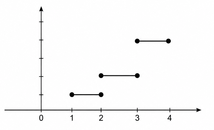
Graph of the cdf of a continuous random variable
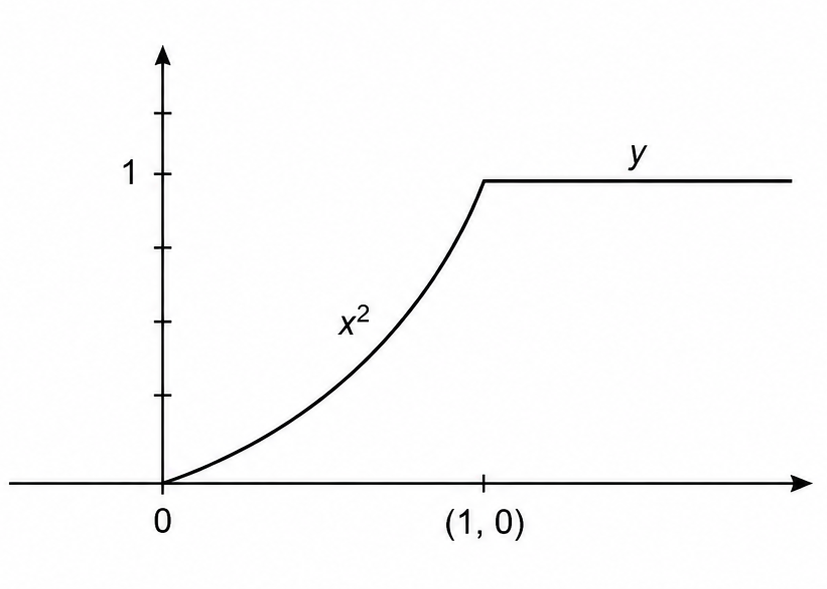
10. If the space of a random variable $X$ consists of the values $x_1 < x_2 < \cdots < x_n$ then
$$f_X(x_i) = F_X(x_i) – F_X(x_{i-1}) \quad \text{for } i = 2, 3, \cdots n$$
Since
$$F_X(x_i) = \sum_{t \leq x_i} f_X(t) \quad \text{and} \quad F_X(x_{i-1}) = \sum_{t \leq x_{i-1}} f_X(t)$$
We have $F_X(x_i) – F_X(x_i – 1)$
$$= [f_X(x_1) + f_X(x_2) + \cdots + f_X(x_i)] – [f_X(x_1) + f_X(x_2) + \cdots + f_X(x_{i-1})]$$
$$= f_X(x_i)$$
Hence proved.
11. $p(X > x_i) = 1 – F_X(x_i) \quad i = 1, 2, 3, \cdots, n$
Since $p(X > x_i) = 1 – p(X \leq x_i)$
$$= 1 – F_X(x_i) \quad i = 1, 2, 3, \cdots, n$$
12. $p(X \geq x_i) = 1 – F_X(x_{i-1}) \quad i = 1, 2, 3, \cdots, n$
Since $p(X \geq x_i) = 1 – p(x < x_i)$
$$= 1 – p(X \leq x_{i-1}) \quad [\because f_X(x) = 0 \ x_{i-1} < x < x_i]$$
$$= 1 – F_X(x_{i-1})$$
In particular $p(x \geq x_i) = 1$.
Inverse Cummulative Distribution Function
If $F_X(x)$ is the cdf of a random variable and is strictly increasing on some interval and that $F_X(x) = 0$ to the left of $I$ and $F_X(x) = 1$ to the right of $I$ then its inverse function $F_X^{-1}(x)$ is defined. This will help us in finding $p^{th}$ quantile of the distribution.
That is the $p^{th}$ quantile or $(100p)$th percentile is defined as a value $x_p$ such that $F_X(x_p) = p$ or $p(X \leq x_p) = p$.
Under the assumption stated above $x_p$ is uniquely determined. Special cases of quantile are $p = \dfrac{1}{2}$ and $\dfrac{1}{4}$ and $\dfrac{3}{4}$. Indeed, if $p = \dfrac{1}{2}$ it is said to be median and if $p = \dfrac{1}{4}$ and $p = \dfrac{3}{4}$ then it is said to be $\textit{lower}$ and $\textit{upper quatiles}$ of $X$. This calculation of quantiles can be either using integration or using the graph of $F_X(x)$.
Example 9
For each of the following find $K$ so that the function can serve as the probability distribution of a random variable.
(a) $f_X(x) = k\left(\dfrac{1}{3}\right)^x \quad x = 1, 2, 3, \cdots$
(b) $f_X(x) = kx^2 \quad x = 1, 2, 3, \cdots, 10$
(c) $f_X(x) = k^x(1-k) \quad x = 0, 1, 2, \cdots$
(a) Since, the space of $X$ is $A = \{1, 2, 3, \cdots\}$, $X$ is discrete.
$$\therefore \quad \sum_x f_X(x) = 1$$
$$\therefore \quad \sum_{x=1}^{\infty} k \left(\frac{1}{3}\right)^x = 1 \implies K\left[ \left(\frac{1}{3}\right) + \left(\frac{1}{3}\right)^2 + \left(\frac{1}{3}\right)^3 + \left(\frac{1}{3}\right)^4 + \cdots \right] = 1 $$
$$\implies K\left(\frac{1}{3}\right)\left[ \frac{1}{1 – (1/3)} \right] = 1$$
$$\implies K\left(\frac{1}{3}\right) \times \left(\frac{3}{2}\right) = 1 \implies K = 2$$
(b) Space of $X$ is $A = \{1, 2, 3, \cdots, 10\}$. $X$ is discrete.
$$\therefore \quad \sum_x f_X(x) = 1 \implies \sum_{x=1}^{10} K x^2 = 1$$
$$\implies K(1^2 + 2^2 + 3^2 + \cdots + 10^2) = 1$$
$$\implies K \frac{10(11)(21)}{6} = 1; \quad K = \frac{1}{385}$$
(c) In this case also $X$ is discrete
$$\therefore \quad \sum_x f_X(x) = 1 \implies \sum_{x=0}^{\infty} K^x(1-K) = 1$$
$$\implies (1-K)\left[1 + K + K^2 + \cdots\right] = 1$$
$$\implies (1-K)\frac{1}{1-K} = 1$$
The above identity exists only for $0 < K < 1$.
$\therefore$ For any $K$ s.t $0 < K < 1$, $f_X(x)$ is an admissable pdf of a discrete random variable $X$.