
Bayesian Tool Kit
In Bayesian analysis, sequential updating refers to the process of continuously updating beliefs about a parameter as new data becomes available. Starting with a prior distribution, data are incorporated to form a posterior distribution, which then serves as the prior for the next round of updating. This iterative process enables adaptive learning as evidence accumulates.
Prior $\rightarrow$ Data $\rightarrow$ Posterior $\rightarrow$ Prior $\rightarrow$ Data $\rightarrow$ Posterior $\cdots \cdots \cdots \cdots$
1. Prior to Posterior Update
We begin with a prior distribution $p(\theta)$, reflecting beliefs about the parameter $\theta$ before any data are observed. Upon observing data, Bayes’ theorem is applied to obtain the posterior distribution $p(\theta \mid \text{X})$:
$$p(\theta \mid \text{X}) = \frac{p(\text{X} \mid \theta)\, p(\theta)}{p(\text{X})}$$
where:
- $p(\text{X} \mid \theta)$ is the likelihood of the data given $\theta$
- $p(\theta)$ is the prior distribution
- $p(\text{X})$ is the marginal likelihood, ensuring the posterior is properly normalized
2. Posterior as the New Prior
Once the posterior is obtained, it reflects the updated belief about $\theta$ after observing the first batch of data. When new data arrive, the posterior from the previous step serves directly as the prior for the next update:
$$p(\theta \mid \text{new data}) = \frac{p(\text{new data} \mid \theta)\, p(\theta \mid \text{previous data})}{p(\text{new data})}$$
This ensures that all previously accumulated information is carried forward into each subsequent update.
3. The Iterative Process
Sequential updating proceeds as follows:
- Begin with a prior $p(\theta)$ based on initial knowledge or assumptions.
- Update to a posterior using the first batch of observed data.
- Use the posterior as the new prior and update again with the next batch of data.
- Repeat as further data arrive.
Each update refines the estimate of $\theta$, yielding progressively more informed inference.
4. Advantages of Sequential Updating
- Flexibility: The model is updated continuously as new data become available, without recomputing from scratch at each stage.
- Real-time learning: The approach is well-suited to settings where data arrive sequentially, such as time-series applications.
- Retention of prior knowledge: By carrying the posterior forward as the new prior, all previously observed information is consistently preserved across updates.
EXAMPLE: SINGLE-ARM PHASE II FUTILITY MONITORING
1. TRIAL DESIGN
Design type:
- Single-arm, open-label, Phase II, Bayesian futility monitoring
- Endpoint: Binary tumor response (responder = 1, non-responder = 0)
- Historical / null response rate (standard of care): $p_0 = 0.15$
- Target / clinically meaningful response rate: $p_1 = 0.35$
- Sample size: $N = 60$ patients, enrolled and analyzed in 6 sequential cohorts of 10 patients each.
Interim looks occur after each fixed block of 10, rather than continuously, to limit operational burden on sites/CRO.
Stopping rule (pre-specified before any data are observed):
- At each interim analysis, compute $\Pr(\theta > p_1 \mid \text{data})$
- If this probability is $< 0.05$ then STOP for FUTILITY; Otherwise, CONTINUE to next cohort
- At the final analysis ($n=60$), declare success if $\Pr(\theta > p_0 \mid \text{data}) > 0.95$
2. THE MODEL
Let $\theta$ denote the true, unknown response rate of the drug.
Likelihood
Each patient outcome $y_i \in \{0,1\}$ is Bernoulli:
$y_i \mid \theta \sim \text{Bernoulli}(\theta)$
For a cohort of $n$ patients with $x$ responders and $f = n-x$ non-responders, the aggregated likelihood is Binomial:
$$x \mid \theta \sim \text{Binomial}(n,\theta)$$
Conjugate posterior update:
With prior $\theta \sim \text{Beta}(a,b)$, observing $x$ successes and $f$ failures gives posterior
$$\theta \mid \text{data} \sim \text{Beta}(a+x, n-x+b)=\theta \mid \text{data} \sim \text{Beta}(a+x, f+b)$$
This composes sequentially: the posterior after cohort $k-1$ becomes the prior for cohort $k$:
$a_k = a_{k-1} + x_k, \qquad b_k = b_{k-1} + f_k$
The posterior after $K$ cohorts is identical whether computed cohort-by-cohort or in one pooled update on $\sum x_k, \sum f_k$.
This is why repeated Bayesian “peeking” at interim data needs no alpha-spending correction, unlike frequentist group-sequential designs.
Posterior summaries at each look
Posterior mean: $$E[\theta \mid \text{data}] = \dfrac{a_k}{a_k+b_k}$$
95% credible interval: $$\left[F^{-1}_{\text{Beta}(a_k,b_k)}(0.025),\ F^{-1}_{\text{Beta}(a_k,b_k)}(0.975)\right]$$
Futility signal:
$$\Pr(\theta > p_1 \mid \text{data}) = 1 – F_{\text{Beta}(a_k,b_k)}(p_1)$$
Success signal:
$$\Pr(\theta > p_0 \mid \text{data}) = 1 – F_{\text{Beta}(a_k,b_k)}(p_0)$$
3. PRIOR CONSTRUCTION – WITH EXPLICIT JUSTIFICATION
A Beta$(a_0,b_0)$ prior has two free parameters and therefore requires two independently justified design choices
Choice 1: Target location statistic:
Prior mean $= p_0 = 0.15$.
Justification: absent trial data, assume the new drug performs like standard of care (“skeptical” prior). This is a modeling convention, not a mathematical necessity – other conventions (flat prior, prior centered between $p_0$ and $p_1$, prior from historical control IPD) are equally legitimate and are used in practice.
Choice 2: Prior strength (effective sample size, $\text{ESS} = a_0+b_0$):
This must be chosen and justified independently of Choice 1. It controls how quickly real data can overwhelm the prior.
Given (mean $m$, ESS $= a_0+b_0$), both parameters are determined by:
$a_0 = m \times \text{ESS}, \qquad b_0 = (1-m)\times \text{ESS}$
Two schemas are presented below, both meeting the “not flat, not overly informative” description used loosely in earlier notes – but each with the two design choices stated explicitly and separately, rather than backed into via an arbitrarily fixed $a_0=1$.
Schema A: Flat / non-informative prior
$a_0 = 1.0,\ b_0 = 1.0$
Mean $= 0.5$, ESS $= 2$
Justification: no informative belief encoded; equivalent to Uniform$(0,1)$. Serves as the reference case – the posterior is driven entirely by observed data from patient 1 onward.
Schema B: Weakly informative, skeptical prior
Target mean $= 0.15$ (Choice 1, as justified above)
Target ESS $= 4$ (Choice 2: deliberately weak – less than half the weight of a single 10-patient cohort)
$a_0 = 0.15 \times 4 = 0.60$ $b_0 = 0.85 \times 4 = 3.40$
This implies, mean $= 0.60/4.0 = 0.150$
Variance $= \dfrac{m(1-m)}{\text{ESS}+1} = \dfrac{0.15\times 0.85}{5} = 0.0255$, SD $\approx 0.160$ (wide – consistent with “weakly informative”)
4. SIMULATED PATIENT-LEVEL DATA
Ground truth used only to generate the data (not known to the analysis):
$\theta_{\text{true}} = 0.30$
outcomes = [0,1,1,0,0,0,0,1,0,1, 0,1,1,0,0,0,0,0,0,0, 0,0,0,0,0,1,0,0,0,0, 0,0,0,1,1,1,0,0,0,0, 0,0,0,1,0,0,0,0,0,0, 1,1,1,1,0,1,0,0,0,0]
Cohort boundaries: [1:10], [11:20], [21:30], [31:40], [41:50], [51:60]
5. SEQUENTIAL POSTERIOR UPDATES UNDER EACH SCHEMA
Schema A: Beta(1.0, 1.0) start
Cohort 1 (x=4,f=6): a=5.0, b=7.0 -> mean=0.4167
Cohort 2 (x=2,f=8): a=7.0, b=15.0 -> mean=0.3182
Cohort 3 (x=1,f=9): a=8.0, b=24.0 -> mean=0.2500
Cohort 4 (x=3,f=7): a=11.0, b=31.0 -> mean=0.2619
Cohort 5 (x=1,f=9): a=12.0, b=40.0 -> mean=0.2308
Cohort 6 (x=5,f=5): a=17.0, b=45.0 -> mean=0.2742
Schema B: Beta(0.60, 3.40) start
Cohort 1 (x=4,f=6): a=4.60, b=9.40 -> mean=0.3286
Cohort 2 (x=2,f=8): a=6.60, b=17.40 -> mean=0.2750
Cohort 3 (x=1,f=9): a=7.60, b=26.40 -> mean=0.2235
Cohort 4 (x=3,f=7): a=10.60, b=33.40 -> mean=0.2409
Cohort 5 (x=1,f=9): a=11.60, b=42.40 -> mean=0.2148
Cohort 6 (x=5,f=5): a=16.60, b=47.40 -> mean=0.2594
NOTE: exact $\Pr(\theta > p_1 \mid \text{data})$ values at each look require evaluating the Beta CDF numerically (e.g. using R or Python) for both schemas.
BETA CDF VIA F-DISTRIBUTION TABLE
Exact relation:
If $\theta \sim \text{Beta}(a,b)$, then $F = \dfrac{b\,\theta}{a(1-\theta)} \sim F_{(2a,\ 2b)}$
So, $\Pr(\theta > p_1) = \Pr\!\left(F_{(2a,2b)} > f_0\right), \qquad f_0 = \dfrac{b}{a}\cdot\dfrac{p_1}{1-p_1}$
Decision rule:
STOP for futility if $f_0 > F_{0.05}(2a,\,2b)$ (the tabulated upper-5% critical value), since that is equivalent to $\Pr(\theta>p_1) < 0.05$.
SCHEMA A: Beta(1,1)
START – integer $a,b$ throughout, so $2a,2b$ are valid table degrees of freedom at every cohort.
$p_1 = 0.35 \Rightarrow \dfrac{p_1}{1-p_1} = 0.5385$
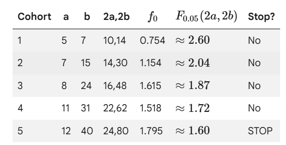
Under Schema A, table-exact futility stop occurs at cohort 5 (n=50).
SCHEMA B FUTILITY CHECK VIA F-TABLE – TWO APPROXIMATION SCHEMES
Relation used throughout:
$$F = \dfrac{b\,\theta}{a(1-\theta)} \sim F_{(2a,\,2b)}$$
$$f_0 = \dfrac{b}{a}\cdot\dfrac{p_1}{1-p_1}, \qquad p_1=0.35 \Rightarrow \dfrac{p_1}{1-p_1}=0.5385$$
Decision: STOP for futility if $f_0 > F_{0.05}(2a,\,2b)$.
Schema B posterior sequence (unrounded), for reference:
C1: a=4.60, b=9.40 | C2: a=6.60, b=17.40 | C3: a=7.60, b=26.40 C4: a=10.60, b=33.40 | C5: a=11.60, b=42.40 | C6: a=16.60, b=47.40
SCHEME 1: INTERPOLATE IN THE F-TABLE (use exact non-integer df)
Compute $2a, 2b$ directly from the unrounded posterior, then read $F_{0.05}(2a,2b)$ by linear interpolation between the nearest tabulated row/column pairs in a standard $F_{0.05}$ table.
Result under Scheme 1: futility triggers at cohort 5, with cohort 3 sitting almost exactly on the boundary – interpolation uncertainty means cohort 3 cannot be called with confidence under this scheme, but cohort 5 clears the threshold unambiguously.
SCHEME 2: ROUND POSTERIOR (a,b) TO NEAREST INTEGERS FIRST
Round $a,b$ to the nearest whole number at each cohort BEFORE forming $2a,2b$, so the resulting degrees of freedom land closer to (though still not always exactly on) standard table entries.
Rounded posterior: C1 (5,9), C2 (7,17), C3 (8,26), C4 (11,33), C5 (12,42), C6 (17,47)
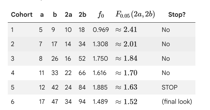
Result under Scheme 2: futility triggers at cohort 5. Cohort 3 is not borderline here (1.750 clearly below 1.84) – rounding removed the ambiguity that Scheme 1 showed at cohort 3.
COMPARISON
Both schemes agree on the stopping cohort: futility triggers at cohort 5 (n=50) under Schema B, matching the Schema A result obtained earlier by the same table method.
They disagree only on cohort 3, where Scheme 1 (unrounded df, interpolated) lands almost exactly on the critical value while Scheme 2 (rounded df) does not flag it. This disagreement is a direct consequence of the approximation method, not of the underlying data – it should be reported as an artifact of table interpolation, not treated as a genuine signal.
All $F_{0.05}$ values above are approximate, read from standard $F$-tables via interpolation; they are not exact analytic values and will vary slightly across different published table editions.
LIMITATIONS
The overall framework used here – Beta-Binomial conjugate futility monitoring in a single-arm Bayesian Phase II design – is standard, current practice in oncology biostatistics, closely following published designs (e.g. Thall & Simon; Lee & Liu) and consistent with FDA guidance on Bayesian and complex-innovative trial designs.
The cohort-based interim look structure is also realistic, reflecting genuine operational preferences over continuous monitoring. However, this case study departs from real practice in one important respect: a real, regulator-facing Statistical Analysis Plan would not rely on a single prior specification run once through the data.
It would report pre-trial simulated operating characteristics (Type I error, power) and a sensitivity analysis showing whether the stopping decision is stable across multiple reasonable prior choices.
Reviewers routinely ask how sensitive a Bayesian design is to its prior, and a single unexamined prior trajectory – as presented in this note – would not satisfy that scrutiny on its own.
HOW THIS MAPS TO A REAL SAP / REAL PRACTICE
- The Beta-Binomial conjugate setup above is essentially what underlies Bayesian single-arm Phase II designs used in oncology (variants of Thall & Simon’s Bayesian designs, and Lee & Liu’s Bayesian optimal designs), and is one of the simplest cases explicitly named in FDA’s Bayesian methodology guidance and the BSA Demonstration Project (“sequential analyses”).
- In a real SAP, you would also pre-specify: the exact futility/efficacy thresholds (here 0.05 / 0.95), the cohort / look schedule, what happens operationally at a “stop” decision (enrollment hold, DSMB review), and simulation-based operating characteristics (Type I error, power) computed by simulating many trials under $\theta=p_0$ and $\theta=p_1$ BEFORE the real trial starts – this calibration step is what FDA reviewers actually scrutinize most closely, even for Bayesian designs.
- The “telescoping” property shown in Section 2 (sequential update = pooled update) is the mathematical reason no alpha-spending correction is applied here, unlike a frequentist group-sequential design with the same 6 looks.
Some More Applications
1. Interim monitoring for early stopping (futility/efficacy)
This is the most common application. At each interim look, the posterior probability of a clinically meaningful effect is recalculated using all data so far, and the trial stops if that probability crosses a pre-specified threshold (e.g., stop for futility if P(effect > MCID | data) < 0.05).
- FDA’s own guidance lists “determining futility or success earlier in adaptive trials” as a standard Bayesian use case, and FDA’s 2026 draft guidance “Use of Bayesian Methodology in Clinical Trials of Drug and Biological Products” explicitly covers using Bayesian calculations to govern the timing and adaptation rules for interim analyses in adaptive designs.
- This is written into actual SAPs as a Bayesian Sequential Probability Ratio Test or posterior-predictive stopping rule, most visibly in medical device trials (FDA’s 2010 device-specific Bayesian guidance predates the drug guidance by 16 years) and in oncology platform trials.
2. Response-adaptive randomization (RAR)
This is where sequential updating isn’t just a monitoring tool but literally drives trial conduct in real time.
- I-SPY2 (breast cancer, neoadjuvant setting): uses Bayesian adaptive randomization to assign more patients to treatments that have performed well for similar patients recruited earlier — data from treated patients are used to update allocation probabilities at each interim analysis. Results were published in NEJM alongside a companion piece by Giovanni Parmigiani explaining the Bayesian vs. frequentist design tradeoffs.
- I-SPY2.2 (the current SMART reconfiguration): uses Thompson sampling to update randomization probabilities at each of up to three treatment stages, based on the posterior probability that a given treatment is part of the optimal regime for pathological complete response. This design demonstrated in 2024 that therapy de-escalation was feasible for several patient subgroups without compromising outcomes — a real clinical conclusion driven by the sequential-update mechanism.
- BATTLE / BATTLE-2 (lung cancer, biomarker-linked): patients were adaptively randomized using emerging data after an initial equal-randomization period, with the same design extended in BATTLE-2 with different drug combinations.
- Berry’s own retrospective analysis of I-SPY2 found that for neratinib, roughly 10 of the 17 percentage-point improvement in pathological complete response over control was attributable to the adaptive randomization mechanism itself, not the drug’s intrinsic effect — i.e., the sequential-update engine measurably changed trial efficiency, not just analysis.
3. COVID-era platform trials
- RECOVERY and REMAP-CAP: these platform trials produced results that directly informed regulatory decisions during the pandemic. REMAP-CAP in particular is a fully Bayesian, perpetually-adapting platform (shared control arm, posterior-driven arm dropping/adding) — it shares the same shared-control, multi-arm architecture as I-SPY2, GBM AGILE, and Precision Promise.
- GBM AGILE (glioblastoma) is another live example of this same shared-control multi-arm Bayesian platform.
4. Sample size / dose-finding via posterior updating
Dose-escalation designs (CRM — Continual Reassessment Method, and its Bayesian variants) sequentially update a dose-toxicity model after each cohort, rather than using fixed 3+3 rules. This is standard in Phase I oncology and is explicitly recognized in FDA’s guidance as informing “design elements (e.g., dose selection) for subsequent clinical trials”.
5. The regulatory infrastructure now built around this
- FDA published a draft guidance in 2025/2026, “Use of Bayesian Methodology in Clinical Trials of Drug and Biological Products,” which is meant to help sponsors use Bayesian calculations for earlier futility/success calls, dose selection, borrowing from external/real-world data, subgroup analysis, and even primary inference. FDA Commissioner Marty Makary specifically framed this as addressing cost and timeline problems in drug development.
- FDA also runs a Bayesian Statistical Analysis (BSA) Demonstration Project where sponsors work directly with FDA on sequential analyses, hierarchical subgroup models, and pediatric borrowing, sharing design details and lessons learned as the trial progresses — this is about as close as you get to a public, semi-authenticated trail of real SAPs using sequential Bayesian updating.
- FDA has tied this formally to ICH E11A and E20 guidances, and the commitment originates from PDUFA VII, so it’s not experimental — it’s now procedural infrastructure sponsors are expected to engage with.
Remarks
- The I-SPY2.2 SMART paper (arXiv 2505.16047, Norwood/Davidian et al.) is a genuinely technical, publicly available writeup of the Thompson-sampling update rule — closest thing to reading an actual “live” sequential-update algorithm used in a real trial.
- FDA’s guidance document itself (“Use of Bayesian Methodology in Clinical Trials of Drug and Biological Products FDA”) is short (~20 pages) and readable, and is the document sponsors now cite in SAPs when justifying Bayesian sequential designs to reviewers.
- BATTLE-2 (Papadimitrakopoulou et al. 2013) and the original I-SPY2 NEJM papers are the most-cited “real trial, real SAP, real regulatory outcome” examples in the literature.
- One nuance worth flagging: even in these designs, sponsors still report frequentist-style operating characteristics (Type I error, power) via simulation to satisfy regulators — FDA emphasizes simulation studies for evaluating operating characteristics even in Bayesian adaptive trials.
- In practice it’s rarely “pure” sequential Bayesian updating in isolation — it’s Bayesian updating as the trial mechanism, wrapped in frequentist-style pre-trial calibration to get regulatory buy-in. That hybrid is basically the norm across all the examples above.
References
1. FDA. “FDA Issues Guidance on Modernizing Statistical Methods for Clinical Trials” (press announcement). https://www.fda.gov/news-events/press-announcements/fda-issues-guidance-modernizing-statistical-methods-clinical-trials
2. FDA. “Use of Bayesian Methodology in Clinical Trials of Drug and Biological Products” (draft guidance). https://www.fda.gov/regulatory-information/search-fda-guidance-documents/use-bayesian-methodology-clinical-trials-drug-and-biological-products
3. FDA. “Guidance Recap Podcast | Use of Bayesian Methodology in Clinical Trials of Drug and Biological Products.” https://www.fda.gov/drugs/guidances-drugs/guidance-recap-podcast-use-bayesian-methodology-clinical-trials-drug-and-biological-products
4. FDA. “Bayesian Statistical Analysis (BSA) Demonstration Project.” https://www.fda.gov/about-fda/cder-center-clinical-trial-innovation-c3ti/bayesian-statistical-analysis-bsa-demonstration-project
5. FDA. “Guidance for the Use of Bayesian Statistics in Medical Device Clinical Trials” (2010).
6. Norwood, P., Yau, C., Wolf, D., Tsiatis, A., Davidian, M. “Bayesian adaptive randomization in the I-SPY2 sequential multiple assignment randomized trial” (I-SPY2.2). arXiv:2505.16047. https://arxiv.org/abs/2505.16047
7. “Re-inventing drug development: A case study of the I-SPY 2 breast cancer clinical trials program.” ResearchGate. https://www.researchgate.net/publication/319619320
8. “I-SPY 2: An Adaptive Breast Cancer Trial Design in the Setting of Neoadjuvant Chemotherapy.” (Barker et al. 2009; Park et al. 2016).
9. Cancer Therapy Advisor. “Adaptive Randomization and the I-SPY 2 Trial Platform” (interview with Giovanni Parmigiani). https://www.cancertherapyadvisor.com/home/cancer-topics/breast-cancer/adaptive-randomization-and-the-i-spy-2-trial-platform/
10. British Journal of Cancer. “A Bayesian adaptive design for biomarker trials with linked treatments.” https://www.nature.com/articles/bjc2015278
11. Papadimitrakopoulou, V. et al. “BATTLE-2” (2013), as referenced in the above BJC article.
12. IntuitionLabs. “Adaptive Trial Design: A Guide to Flexible Clinical Trials.” https://intuitionlabs.ai/articles/adaptive-clinical-trial-design
13. “Using Bayesian Statistics in Confirmatory Clinical Trials in the Regulatory Setting.” arXiv:2311.16506. https://arxiv.org/pdf/2311.16506
14. “Bayesian Sequentially Monitored Multi-arm Experiments with Multiple Comparison Adjustments.” arXiv:1608.08076. https://arxiv.org/pdf/1608.08076
15. “Estimating Design Operating Characteristics in Bayesian Adaptive Clinical Trials.” arXiv:2105.03022. https://arxiv.org/pdf/2105.03022
16. Bayesian Spectacles. “A Bayesian Perspective on the Proposed FDA Guidelines for Adaptive Clinical Trials.” https://www.bayesianspectacles.org/a-bayesian-perspective-on-the-proposed-fda-guidelines-for-adaptive-clinical-trials/
17. Statistical Modeling, Causal Inference, and Social Science (blog). “FDA guidance on Bayesian clinical trials.” https://statmodeling.stat.columbia.edu/2026/01/15/fda-guidance-on-bayesian-clinical-trials/